6.5: Quantum Numbers, Atomic Orbitals, and Electron Configurations

Timothy Minger, Ph.D.

6.5: Quantum Numbers, Atomic Orbitals, and Electron Configurations

Learning Objective

Represent the organization of electrons by an electron configuration and orbital diagram.

The flight path of a commercial airliner is carefully regulated by the Federal Aviation Administration. Each airplane must maintain a distance of five miles from another plane flying at the same altitude and 2,000 feet above and below another aircraft (1,000 feet if the altitude is less than 29,000 feet). So, each aircraft only has certain positions it is allowed to maintain while it flies. As we explore quantum mechanics, we see that electrons have similar restrictions on their locations.

Quantum Numbers

We use a series of specific numbers, called quantum numbers, to describe the location of an electron in an associated atom. Quantum numbers specify the properties of the atomic orbitals and the electrons in those orbitals. An electron in an atom or ion has four quantum numbers to describe its state. Think of them as important variables in an equation that describe the three-dimensional position of electrons in a given atom.

Principal Quantum Number $(n)$

The principal quantum number, signified by $n$ , is the main energy level occupied by the electron. Energy levels are fixed distances from the nucleus of a given atom. They are described in whole number increments (e.g., 1, 2, 3, 4, 5, 6, …). At location $n = 1$ , an electron would be closest to the nucleus, while at $n = 2$ the electron would be farther, and at $n = 3$ farther yet. As we will see, the principal quantum number corresponds to the row (period) number for an atom on the periodic table.

Angular Momentum Quantum Number $(l)$

The angular momentum quantum number, signified by $l$ , describes the general region an electron occupies—its orbital shape. The value of $(l)$ depends on the value of the principal quantum number, $n$ . The angular momentum quantum number can have positive values of zero to $(n - 1)$ . If $n = 2$ $(l)$ could be either $0$ or $1$ .

Magnetic Quantum Number $(m_{l})$ _$(l)$ $(m_{l})$

The magnetic quantum number, signified as $m_{l}$ , describes the orbital orientation in space. Electrons can be situated in one of three planes in three dimensional space around a given nucleus ( $x$ , $y$ , and $z$ ). For a given value of the angular momentum quantum number, $(l)$ , there can be $(2 l + 1)$ values for $m_{l}$ . For example:

n = 2

$(l)$ = 0 or 1

for $(l)$ = 0, m_$(l)$ = 0

for = 1, m_$(l)$ = -1, 0, +1

Table 6.5.1: Principal Energy Levels and Sublevels

Principal Energy Level

Number of Possible Sublevels

Possible Angular Momentum of Quantum Numbers

Orbital Designation by Principal Energy Level and Sublevel

n = 1

1

(l)

= 0

1s

n = 2

2

(l)

= 0

2s

(l)

= 1

2p

n = 3

3

(l)

= 0

3s

(l)

= 1

3p

(l)

= 2

3d

n = 4

4

(l)

= 0

4s

(l)

= 1

4p

(l)

= 2

4d

(l)

= 3

4f

Table 6.5.1 shows the possible angular momentum quantum number values $(l)$ for the corresponding principal quantum numbers $(n) o f \(n = 1, n = 2, n = 3,$ and $n = 4$

Spin Quantum Number $(m_{s})$

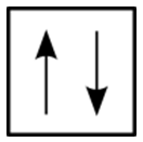
The spin quantum number describes the spin for a given electron. An electron can have one of two associated spins, (+[latex]\frac{1}{2}[/latex]) spin, or (-[latex]\frac{1}{2}[/latex]) spin. An electron cannot have zero spin. We also represent spin with arrows ↑ or ↓. A single orbital can hold a maximum of two electrons, and each must have an opposite spin.

Orbitals

We can apply our knowledge of quantum numbers to describe the arrangement of electrons for a given atom. We do this with something called electron configurations. They are effectively a map of the electrons for a given atom. We look at the four quantum numbers for a given electron and then assign that electron to a specific orbital below.

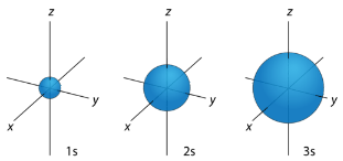
s Orbitals

For any value of $n$ , a value of $l = 0$ places an electron in an $s$ orbital. This orbital is spherical in shape:

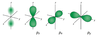
Graphic depiction of the s orbital on an x, y, z plane — *Figure 6.5.1:* s orbitals have no orientational preference and resemble spheres.

p Orbitals

For the table below, we see that we can have three possible orbitals when $l = 1$ . These are designated as $p$ orbitals and have dumbbell shapes. Each of the $p$ orbitals has a different orientation in three-dimensional space.

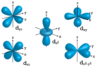
Graphic depiction of the p orbital on an x, y, z plane — *Figure 6.5.2:* p orbitals resemble dumbbells and can be oriented in one of three directions (along the x, y, or z axis of a coordinate system).

d Orbitals

When $l = 2$ , $m_{l}$ values can be $- 2, - 1, 0, + 1, + 2$ for a total of five $d$ orbitals. Note that all five of the orbitals have specific three-dimensional orientations.

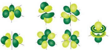
Graphic depiction of the d orbital on an x, y, z plane — *Figure 6.5.3:* d orbitals have an orientational preference and exhibit complex structures.

f Orbitals

The most complex orbitals are the $f$ orbitals. When $l = 3$ , $m_{l}$ values can be $- 3, - 2, - 1, 0, + 1, + 2, + 3$ for a total of seven different orbital shapes. Again, note the specific orientations of the different $f$ orbitals.

Orbitals that have the same value of the principal quantum number form a shell. Orbitals within a shell are divided into subshells that have the same value of the angular quantum number. Some of the allowed combinations of quantum numbers are compared in Table 6.5.2.

Table 6.5.2: Electron Arrangement Within Energy Levels

Principal Quantum Number (n)	Allowable Sublevels	Number of Orbitals per Sublevel	Number of Orbitals per Principal Energy Level	Number of Electrons per Sublevel	Number of Electrons per Principal Energy Level
1	s	1	1	2	2
2	s	1	4	2	8
2	p	3	4	6	8
3	s	1	9	2	18
	p	3		6
	d	5		10
4	s	1	16	2	32
	p	3		6
	d	5		10
	f	7		14

Electron Configurations

Can you name one thing that easily distinguishes you from the rest of the world? And we’re not talking about DNA—that’s a little expensive to sequence. For many people, it is their email address. Your email address allows people all over the world to contact you. It does not belong to anyone else, but serves to identify you. Electrons also have a unique set of identifiers in the quantum numbers that describe their location and spin. Chemists use an electronic configuration to represent the organization of electrons in shells and subshells in an atom. An electron configuration simply lists the shell and subshell labels, with a right superscript giving the number of electrons in that subshell. The shells and subshells are listed in the order of filling. Electrons are typically organized around an atom by starting at the lowest possible quantum numbers first, which are the shells-subshells with lower energies.

For example, an H atom has a single electron in the 1s subshell. Its electron configuration is:

$H : 1 s^{1}$

He has two electrons in the 1s subshell. Its electron configuration is:

He : 1s²

The three electrons for Li are arranged in the 1s subshell (two electrons) and the 2s subshell (one electron). The electron configuration of Li is:

$Li : 1 s^{2} 2 s^{1}$

Be has four electrons, two in the 1s subshell and two in the 2s subshell. Its electron configuration is:

$Be : 1 s^{2} 2 s^{2}$

Now that the 2s subshell is filled, electrons in larger atoms must go into the 2p subshell, which can hold a maximum of six electrons. The next six elements progressively fill up the 2p subshell:

B: 1s²2s²2p¹
C: 1s²2s²2p²
N: 1s²2s²2p³
O: 1s²2s²2p⁴
F: 1s²2s²2p⁵
Ne: 1s²2s²2p⁶

Now that the 2p subshell is filled (all possible subshells in the n = 2 shell), the next electron for the next-larger atom must go into the n = 3 shell, s subshell.

Second Period Elements

Periods refer to the horizontal rows of the periodic table. Looking at a periodic table you will see that the first period contains only the elements hydrogen and helium. This is because the first principal energy level consists of only the $s$ sublevel and so only two electrons are required in order to fill the entire principal energy level. Each time a new principal energy level begins, as with the third element lithium, a new period is started on the periodic table. As one moves across the second period, electrons are successively added. With beryllium $(Z = 4)$ , the $2 s$ sublevel is complete and the $2 p$ sublevel begins with boron $(Z = 5)$ . Since there are three $2 p$ orbitals and each orbital holds two electrons, the $2 p$ sublevel is filled after six elements. Table 6 $12.5. 1$ shows the electron configurations of the elements in the second period.

Table 6.5.3: Second Period Elements, Symbol, Atomic Number, and Electron Configurations

Element Name

Symbol

Atomic Number

Electron Configuration

Lithium

Li

3

Li : 1 s^{2} 2 s^{1}

Beryllium

Be

4

Li : 1 s^{2} 2 s^{1}

Boron

B

5

1s²2s²2p¹

Carbon

C

6

1s²2s²2p²

Nitrogen

N

7

1s²2s²2p³

Oxygen

O

8

1s²2s²2p⁴

Fluorine

F

9

1s²2s²2p⁵

Neon

Ne

10

1s²2s²2p⁶

Aufbau Principle

Construction of a building begins at the bottom. The foundation is laid and the building goes up step by step. You obviously cannot start with the roof since there is no place to hang it. The building goes from the lowest level to the highest level in a systematic way. In order to create ground state electron configurations for any element, it is necessary to know the way in which the atomic sublevels are organized in order of increasing energy. Figure 6.5.5 shows the order of increasing energy of sublevels.

The lowest energy sublevel is always the $1 s$ sublevel, which consists of one orbital. The single electron of the hydrogen atom will occupy the $1 s$ orbital when the atom is in its ground state. As we proceed with atoms with multiple electrons, those electrons are added to the next lowest sublevel: $2 s$ , $2 p$ , $3 s$ , and so on. The Aufbau principle states that electrons occupy orbitals in order from lowest energy to highest. The Aufbau (German: “building up, construction”) principle is sometimes referred to as the “building up” principle. It is worth noting that in reality atoms are not built by adding protons and electrons one at a time, and that this method is merely an aid for us to understand the end result.

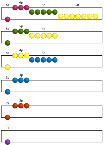
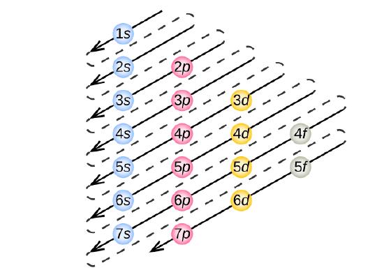
Graph depicting atomic orbitals as they relate to the Aufbau principle, low on the bottom to high energy at the top — Figure 6.5.5: : Electrons are added to atomic orbitals in order from low energy (bottom of the graph) to high (top of the graph) according to the Aufbau principle. Principle energy levels are color coded, while sublevels are grouped together and each circle represents an orbital capable of holding two electrons.

As seen in the figure above, the energies of the sublevels in different principal energy levels eventually begin to overlap. After the $3 p$ sublevel, it would seem logical that the $3 d$ sublevel should be the next lowest in energy. However, the $4 s$ sublevel is slightly lower in energy than the $3 d$ sublevel and thus fills first. Following the filling of the $3 d$ sublevel is the $4 p$ , then the $5 s$ and the $4 d$ . Note that the $4 f$ sublevel does not fill until just after the $6 s$ sublevel. Figure 6 $12.5. 6$ is a useful and simple aid for keeping track of the order of fill of the atomic sublevels.

Chart depicting subshell order for electron configurations s, p, d, f — Figure 6.5.6: The arrow leads through each subshell in the appropriate filling order for electron configurations. This chart is straightforward to construct. Simply make a column for all the s orbitals with each n shell on a separate row. Repeat for p, d, and f. Be sure to only include orbitals allowed by the quantum numbers (no 1p or 2d, and so forth). Finally, draw diagonal lines from top to bottom as shown.

Example 6.5.1: Nitrogen Atoms

Nitrogen has 7 electrons. Write the electron configuration for nitrogen.

Solution

Take a close look at Figure 6.5.5, and use it to figure out how many electrons go into each sublevel, and also the order in which the different sublevels get filled.

1. Begin by filling up the 1s sublevel. This gives 1s². Now all of the orbitals in the red n = 1 block are filled.

2. Next, fill the 2s sublevel. This gives 1s²2s². Now all of the orbitals in the s sublevel of the orange n = 2 block are filled.

3. Notice that we haven’t filled the entire n = 2 block yet… there are still the p orbitals!

The overall electron configuration is: 1s²2s²2p³.

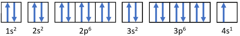
Example 6.5.2: Potassium Atoms

Potassium has 19 electrons. Write the electron configuration code for potassium.

Solution

This time, take a close look at Figure 6.5.5.

1. Begin by filling up the 1s sublevel. This gives 1s². Now the n = 1 level is filled.

2. Next, fill the 2s sublevel. This gives 1s²2s²

3. Next, fill the 2p sublevel. This gives 1s²2s²2p⁶. Now the n = 2 level is filled.

4. Next, fill the 3s sublevel. This gives 1s²2s²2p⁶3s²

5. Next, fill the 3p sublevel. This gives 1s²2s²2p⁶3s²3p⁶

Here’s where we have to be careful – right after 3p⁶!

6. The final electron goes into the 4s sublevel. This gives 1s²2s²2p⁶3s²3p⁶4s¹

The overall electron configuration is: 1s²2s²2p⁶3s²3p⁶4s¹

Exercise 6.5.1: Magnesium and Sodium Atoms

Pauli Exclusion Principle

When we look at the orbital possibilities for a given atom, we see that there are different arrangements of electrons for each different type of atom. Since each electron must maintain its unique identity, we intuitively sense that the four quantum numbers for any given electron must not match up exactly with the four quantum numbers for any other electron in that atom.

For the hydrogen atom, there is no problem since there is only one electron in the $H$ atom. However, when we get to helium we see that the first three quantum numbers for the two electrons are the same: same energy level, same spherical shape. What differentiates the two helium electrons is their spin. One of the electrons has a $+ \frac{1}{2}$ spin while the other electron has a $- \frac{1}{2}$ spin. So the two electrons in the $1 s$ orbital are each unique and distinct from one another because their spins are different. This observation leads to the Pauli exclusion principle, which states that no two electrons in an atom can have the same set of four quantum numbers. The energy of the electron is specified by the principal, angular momentum, and magnetic quantum numbers. If those three numbers are identical for two electrons, the spin numbers must be different in order for the two electrons to be differentiated from one another. The two values of the spin quantum number allow each orbital to hold two electrons. Figure 6. $12.5. 7$ shows how the electrons are indicated in a diagram.

Orbital filling diagram — Figure 6.5.7: In an orbital filling diagram, a square represents an orbital, while arrows represent electrons. An arrow pointing upward represents one spin direction, while an arrow pointing downward represents the other spin direction.

Hund’s Rule

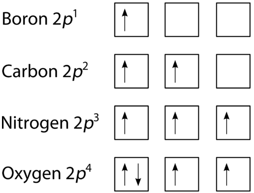
The last of the three rules for constructing electron arrangements requires electrons to be placed one at a time in a set of orbitals within the same sublevel. This minimizes the natural repulsive forces that one electron has for another. Hund’s rule states that orbitals of equal energy are each occupied by one electron before any orbital is occupied by a second electron and that each of the single electrons must have the same spin. The figure below shows how a set of three $p$ orbitals is filled with one, two, three, and four electrons.

Orbital Filling Diagrams

An orbital filling diagram is the more visual way to represent the arrangement of all the electrons in a particular atom. In an orbital filling diagram, the individual orbitals are shown as circles, squares, or horizontal lines. Orbitals within a sublevel are drawn next to each other horizontally. Each sublevel is labeled by its principal energy level and sublevel. Electrons are indicated by arrows: an arrow pointing upwards indicates one spin direction, while a downward pointing arrow indicates the other direction. The orbital filling diagrams for hydrogen, helium, and lithium are shown in the figure below.

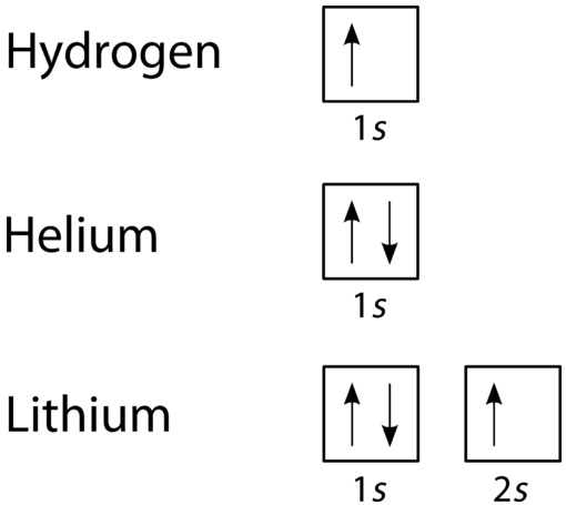
According to the Aufbau process, sublevels and orbitals are filled with electrons in order of increasing energy. Since the $s$ sublevel consists of just one orbital, the second electron simply pairs up with the first electron as in helium. The next element is lithium and necessitates the use of the next available sublevel, the $2 s$ .

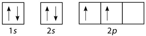
The filling diagram for carbon is shown in Figure 6 $12.5. 10$ . There are two $2 p$ electrons for carbon and each occupies its own $2 p$ orbital.

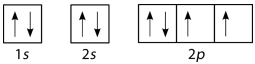
*Figure 6.5.10: Orbital filling diagram for carbon.*

Oxygen has four $2 p$ electrons. After each $2 p$ orbital has one electron in it, the fourth electron can be placed in the first $2 p$ orbital with a spin opposite that of the other electron in that orbital.

*Figure 6.5.11: Orbital filling diagram for oxygen.*

If you keep your papers in manila folders, you can pick up a folder and see how much it weighs. If you want to know how many different papers (articles, bank records, or whatever else you keep in a folder), you have to take everything out and count. A computer directory, on the other hand, tells you exactly how much you have in each file. We can get the same information on atoms. If we use an orbital filling diagram, we have to count arrows. When we look at electron configuration data, we simply add up the numbers.

Example 6.5.3: Carbon Atoms

Draw the orbital filling diagram for carbon and write its electron configuration.

Solution

Step 1: List the known quantities and plan the problem.

Known

Atomic number of carbon, Z = 6

Use the order of fill diagram to draw an orbital filling diagram with a total of six electrons. Follow Hund’s rule. Write the electron configuration.

Step 2: Construct the diagram.

Electron configuration 1s²2s²2p²

Step 3: Think about your result.

Following the 2s sublevel is the 2p, and p sublevels always consist of three orbitals. All three orbitals need to be drawn even if one or more is unoccupied. According to Hund’s rule, the sixth electron enters the second of those p orbitals and has the same spin as the fifth electron.

Exercise 6.5.2: Electronic Configurations

Write the electron configurations and orbital diagrams for

Potassium atom: K
Arsenic atom: As
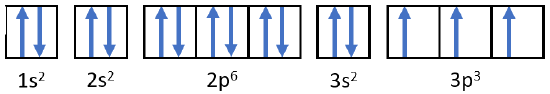
Phosphorus atom: P

Answer

Potassium: 1s²2s²2p⁶3s²3p⁶4s¹

Arsenic: 1s²2s²2p⁶3s²3p⁶4s²3d¹⁰4p³

Phosphorus: 1s²2s²2p⁶3s²3p³

*Orbital filling diagram for phosphorus*

The Atom Neighborhood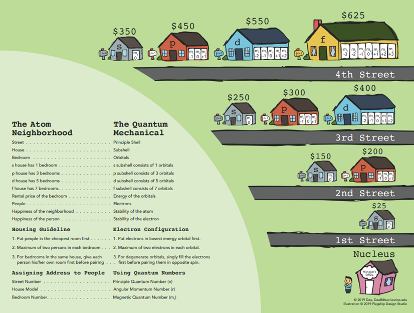Figure 6.5.12 The atom neighborhood. Source: Dr. Binh Dao, Sacramento City College.

Key Takeaways

Quantum numbers specify the arrangements of electrons in orbitals. There are four quantum numbers that provide information about various aspects of electron behavior.
There are four different classes of electron orbitals. These orbitals are determined by the value of the angular momentum quantum number ℓ. An orbital is a wave function for an electron defined by the three quantum numbers, n, ℓ and m_ℓ. Orbitals define regions in space where you are likely to find electrons. s orbitals (ℓ = 0) are spherical shaped. p orbitals (ℓ = 1) are dumb-bell shaped. The three possible p orbitals are always perpendicular to each other.
Electron configuration notation simplifies the indication of where electrons are located in a specific atom. Superscripts are used to indicate the number of electrons in a given sublevel.
The Aufbau principle gives the order of electron filling in an atom. It can be used to describe the locations and energy levels of every electron in a given atom.
Hund’s rule specifies the order of electron filling within a set of orbitals. Orbital filling diagrams are a way of indicating electron locations in orbitals.
The Pauli exclusion principle specifies limits on how identical quantum numbers can be for two electrons in the same atom.

Supplemental Video Support

Vocabulary

Principal quantum number (n): Defines the energy level of the wave function for an electron, the size of the electron’s standing wave, and the number of nodes in that wave.

Quantum numbers: Integer numbers assigned to certain quantities in the electron wave function. Because electron standing waves must be continuous and must not “double over” on themselves, quantum numbers are restricted to integer values.

Contributions & Attributions

Marisa Alviar-Agnew (Sacramento City College)
Henry Agnew (UC Davis)
Paul Flowers (University of North Carolina – Pembroke), Klaus Theopold (University of Delaware) and Richard Langley (Stephen F. Austin State University) with contributing authors. Textbook content produced by OpenStax College is licensed under a Creative Commons Attribution License 4.0 license. Download for free at http://cnx.org/contents/85abf193-2bd…a7ac8df6@9.110).

License

Icon for the Creative Commons Attribution-NonCommercial 4.0 International License

Quantum Numbers

Principal Quantum Number (n)

Angular Momentum Quantum Number (l )

Magnetic Quantum Number (ml )

Spin Quantum Number (ms)

Orbitals

s Orbitals

p Orbitals

d Orbitals

f Orbitals

Electron Configurations

Second Period Elements

Aufbau Principle

Pauli Exclusion Principle

Hund’s Rule

Orbital Filling Diagrams

The Atom NeighborhoodFigure 6.5.12 The atom neighborhood. Source: Dr. Binh Dao, Sacramento City College.

Supplemental Video Support

Vocabulary

Contributions & Attributions

License

Share This Book

Principal Quantum Number $(n)$

Angular Momentum Quantum Number $(l)$

Magnetic Quantum Number $(m_{l})$ _$(l)$ $(m_{l})$

Spin Quantum Number $(m_{s})$