
Section S.5 – The Normal Distribution and The Empirical Rule
The Normal Distribution
Although the characteristics of the population (population parameters) may be unknown, random sampling can be used to yield reliable estimates of these characteristics. Sample data can be plotted on graphs (like histograms or boxplots) to provide a visual representation of the distribution of data values.
Take, for example, the heights of all of the women at MCC. If we were to take a random sample of female MCC students and record their heights, we would most likely find the majority of the heights would be close to a central value, the mean, with larger or smaller values becoming less and less common. The resulting distribution might look something like this:
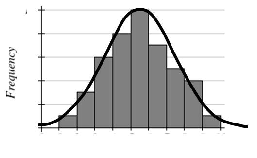
This type of symmetric, bell-shaped distribution is more formally called the Normal Distribution. Because actual data are almost never exactly normally distributed, we say that the data are approximately normal.
| The Normal Distribution |
|
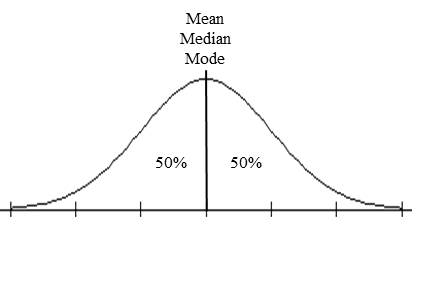
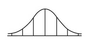
Here are a few important characteristics of the Normal Distribution:
Each tick mark on the horizontal axis is marking off increments of 1 standard deviation above or below the mean. |
| Example 1 |
|
The test scores on a math exam are approximately normally distributed with mean 72 and standard deviation 8. Draw the associated normal distribution curve, and label the axis appropriately. |
|
Since the test scores are approximately normally distributed, we know that the curve is bell-shaped, and centered at its mean of 72. Since the standard deviation is 8, each line on the horizontal axis is 8 units away from the other lines.
48 56 64 72 80 88 96 When drawing a normal distribution curve, we usually extend the curve out to three standard deviations below the mean, and three standard deviations above the mean. |

| You Try S.5.A |
|
Draw the normal distribution curve for the variable X that is approximately normally distributed with mean 15 and standard deviation 2. |
The Empirical Rule
Consider the distributions shown below:
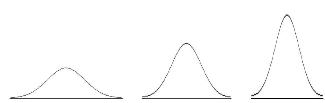
All of them are normally distributed, but each has different variation (spread).
For a Normal Distribution, we use the standard deviation to describe the variation, or spread of the data values around the mean. The standard deviation is commonly represented by the lowercase Greek letter sigma, σ.
While each of the above distributions has a different variation, the proportion (or percentage) of the variation is still distributed in the same way for every normal distribution. That may be a bit confusing, but think about the way percentages work. Perhaps you are leaving a tip for a dinner bill, and you always leave a 20% tip. The dollar amount of the tip will be different for a $100 dinner bill than it would be for a $50 dinner bill, but in either case you would still leave 20% for the tip.
In the three normal distributions above, the variation is different for each of the 3 curves, but the percentage of the variation that is spread throughout the curve is still organized in the same way. The way the variation is distributed in the curve follows what we call the Empirical Rule (also called the 68-95-99.7 Rule).
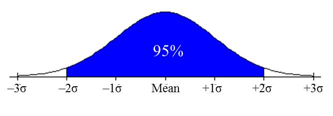
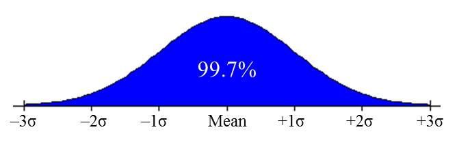
| The Empirical Rule (68-95-99.7 Rule) |
|
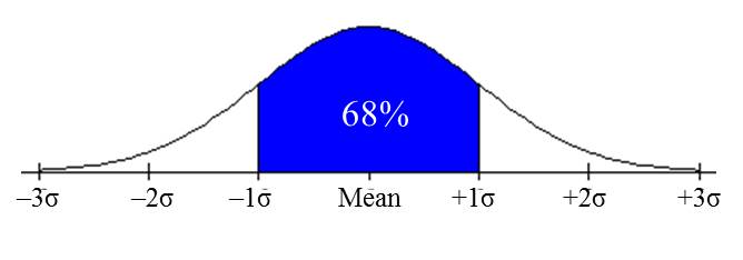
In a normal distribution:
This rule is called the Empirical Rule, sometimes called the “68-95-99.7 Rule”. |
| Example 2 |
|
Scores on a standardized test were normally distributed with a mean of 510 and a standard deviation of 95. Use the Empirical Rule to complete following statements. a. 68% of the students taking this exam scored between _____ and _____. b. 95% of the students taking this exam scored between _____ and _____. c. 99.7% of the students taking this exam scored between _____ and _____. |
|
You will need to make some calculations. Find the mean: 510. Mean + 1 standard deviation = 510 + 95 = 605 Mean + 2 standard deviation = 510 + 2(95) = 700 Mean + 3 standard deviation = 510 + 3(95) = 795 Mean – 1 standard deviation = 510 – 95 = 415 Mean – 2 standard deviation = 510 – 2(95) = 320 Mean – 3 standard deviation = 510 – 3(95) = 225 When answering questions like this, it is helpful to draw and label a sketch of the distribution.
Applying the Empirical Rule, we know that a. 68% of the scores will be within one standard deviation of the mean, so 68% of the students taking this exam scored between 415 and 605. b. 95% of the scores will be within two standard deviations of the mean, so 95% of the students taking this exam scored between 320 and 700. c. 99.7% of the scores will be within three standard deviations of the mean, so 99.7% of the students taking this exam scored between 225 and 795. |

| You Try S.5.B |
|
Gear circumferences for a manufactured bicycle part were normally distributed with a mean of 34 inches and a standard deviation of 0.04 inches. a. Draw and label a sketch of this distribution. b. Use the Empirical Rule to complete following statements. 68% of the students taking this exam scored between _____ and _____. 95% of the students taking this exam scored between _____ and _____. 99.7% of the students taking this exam scored between _____ and _____. |
Section S.5 Answers to You Try Problems
S.5.A
9 11 13 15 17 19 21
S.5.B.
a.

33.88 33.92 33.96 34 34.04 34.08 34.12
b.
68% of the gears have circumferences between 33.96 and 34.04 inches
95% of the gears have circumferences between 33.92 and 34.08 inches
99.7% of the gears have circumferences between 33.88 and 34.12 inches
