Section S.4 - Measures of Variation; Quartiles, Five Number Summary, and Boxplots
Measures of Variation
Another component of describing a data set is how much “Spread” there is in the data set. In other words, how much the data in the distribution vary from one another. It may seem like once we know the center of a data set, we know everything there is to know. The first example will demonstrate why we need measures of variation (or spread).
There are several ways to measure this "Spread" of the data. The three most common measures are the range, standard deviation, and quartiles. In this section we will learn about the range and standard deviation. We will discuss quartiles in the following section.
We will focus first on the simplest measure of spread, called the range.
| Range |
| The range is the difference between the maximum value and the minimum value of the data set. |
|
Example 1 |
|
Consider these three sets of quiz scores: Section A: 5 5 5 5 5 5 5 5 5 5 All three of these sets of data have a mean of 5 and median of 5. If we only calculated a measure of center for each set of scores, we would say the three sets are all identical, yet the sets of scores are clearly quite different. Calculating a measure of variability (or spread) will help identify how they are different. For section A, the range is 0 since both maximum and minimum are 5 and 5 – 5 = 0 For section B, the range is 10 since 10 – 0 = 10 For section C, the range is 2 since 6 – 4 = 2 |
In example 1, the range seems to be revealing how spread out the data is. However, suppose we add a fourth section, Section D.
This section also has a mean and median of 5. The range is 10, yet this data set is quite different than Section B. To better illuminate the differences, we’ll have to turn to more sophisticated measures of variation.
|
You Try S.4.A |
|
The price of a jar of peanut butter at 5 stores was: $3.29, $3.59, $3.79, $3.75, and $3.99. Find the range of the prices. |
| Standard Deviation |
|
The standard deviation is a measure of variation based on measuring how far, on average, each data value deviates, or is different, from the mean. A few important characteristics:
|
Using the data from Section D: 0 5 5 5 5 5 5 5 5 10, we could compute for each data value the difference between the data value and the mean. This will give us an idea of “how far” each value in the data set lies away from the mean.
| data value | deviation: data value - mean |
| 0 | 0-5 = -5 |
| 5 | 5-5 = 0 |
| 5 | 5-5 = 0 |
| 5 | 5-5 = 0 |
| 5 | 5-5 = 0 |
| 5 | 5-5 = 0 |
| 5 | 5-5 = 0 |
| 5 | 5-5 = 0 |
| 5 | 5-5 = 0 |
| 10 | 10-5 = 5 |
We would like to get an idea of the "average" deviation from the mean, but if we find the average of the values in the second column the negative and positive values cancel each other out (this always happens), so instead we square every value in the second column:
|
data value |
deviation: data value - mean |
deviation squared |
|
0 |
0-5 = -5 |
(-5)2 = 25 |
|
5 |
5-5 = 0 |
02 = 0 |
|
5 |
5-5 = 0 |
02 = 0 |
|
5 |
5-5 = 0 |
02 = 0 |
|
5 |
5-5 = 0 |
02 = 0 |
|
5 |
5-5 = 0 |
02 = 0 |
|
5 |
5-5 = 0 |
02 = 0 |
|
5 |
5-5 = 0 |
02 = 0 |
|
5 |
5-5 = 0 |
02 = 0 |
|
10 |
10-5 = 5 |
(5)2 = 25 |
We then add the squared deviations up to get 25 + 0 + 0 + 0 + 0 + 0 + 0 + 0 + 0 + 25 = 50. Ordinarily we would then divide by the number of scores, n, (in this case, 10) to find the mean of the deviations. But we only do this if the data set represents a population; if the data set represents a sample (as it almost always does), we instead divide by n - 1 (in this case, 10 - 1 = 9).11
So in our example, we would have 50/10 = 5 if section D represents a population and 50/9 = about 5.56 if section D represents a sample. These values (5 and 5.56) are called, respectively, the population variance and the sample variance for section D.
Variance can be a useful statistical concept, but note that the units of variance in this instance would be points-squared since we squared all of the deviations. What are points-squared? Good question. We would rather deal with the units we started with (points in this case), so to convert back we take the square root and get:
population standard deviation = [latex]\sqrt{\frac{50}{10}}[/latex] = [latex]\sqrt{5}[/latex] ≈ 2.2
or
sample standard deviation = [latex]\sqrt{\frac{50}{9}}[/latex] ≈ 2.4
If we are unsure whether the data set is a sample or a population, we will usually assume it is a sample, and we will round answers to one more decimal place than the original data, as we have done above.
| To Compute Standard Deviation |
|
To Compute Standard Deviation (Sx): 1. Find the deviation of each data from the mean. In other words, subtract the mean (x̅) from the data value (x). 2. Square each deviation. ( (x - x̅)2 ) 3. Add the squared deviations. ( ∑(x - x̅)2 ) 4. Divide by n, the number of data values, if the data represents a whole population; divide by n – 1 if the data is from a sample. [latex](~\frac{\sum(x~-~\bar{x})^2}{n~-~1}~)[/latex] 5. Compute the square root of the result. Sx = [latex]\sqrt{(~\frac{\sum(x~-~\bar{x})^2}{n~-~1}~)}[/latex] Note: The sigma symbol, ∑, is a mathematical abbreviation that means “Sum of/Add” |
| Example 2 | |||||||||||||||||||||||||||||||||
|
Computing the standard deviation for Section B above, we first calculate that the mean is 5. Using a table can help keep track of your computations for the standard deviation:
Assuming this data represents a population, we will add the squared deviations, divide by 10, the number of data values, and compute the square root: [latex]\sqrt{\frac{25~+~25~+~25~+~25~+~25~+~25~+~25~+~25~+~25~+~25}{10}}[/latex] = [latex]\sqrt{\frac{250}{10}}[/latex] = 5 Notice that the standard deviation of this data set is much larger than that of section D since the data in this set is more spread out. |
For comparison, the standard deviations of all four sections are:
|
Section A: 5 5 5 5 5 5 5 5 5 5 |
Standard deviation: 0 |
|
Section B: 0 0 0 0 0 10 10 10 10 10 |
Standard deviation: 5 |
|
Section C: 4 4 4 5 5 5 5 6 6 6 |
Standard deviation: 0.8 |
|
Section D: 0 5 5 5 5 5 5 5 5 10 |
Standard deviation: 2.2 |
| You Try S.4.B |
|
The price of a jar of peanut butter at 5 stores were: $3.29, $3.59, $3.79, $3.75, and $3.99. Find the standard deviation of the prices. |
| Calculator Instructions for Finding Summary Statistics Using TI-83/84 |
1. Turn on the calculator
2. Press the “STAT” key
3. Hit “Enter” on option 1: “Edit”
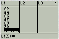
This will bring you to a screen that contains lists: L1, L2, L3, etc.
3. Enter the data values (one value per row) into L1. For any negative values you need to use the (-) key, not the subtraction key. Continue until all data is entered into L1.
4. Press the “STAT” key again
5. Use the arrow key to scroll over to “CALC”.
6. Select option 1: “1-Var Stats”
7. Indicate that the data is in L1 (2nd, then 1 for L1)|
8. Scroll down to “Calculate” and hit “Enter”
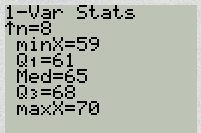
The summary statistics should now be displayed. You may scroll down with your arrow key to get remaining statistics. Using “1-Var Stats” you can get the sample mean, sample standard deviation, population standard deviation, and 5 number summary.
| Example 3 | |||||||||||||||||||||||||||||||||
|
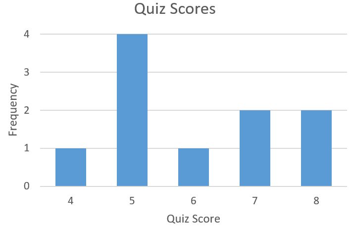
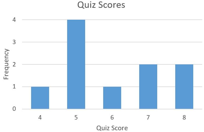
Find the range and standard deviation for the quiz scores. If necessary, round to the nearest hundredth.
Range = maximum value – Minimum value Range = 8 – 4 = 4 Standard Deviation
[latex]\sqrt{\frac{18}{10~-~1}}[/latex] = [latex]\sqrt{2}[/latex] = 1.414213562 Standard Deviation is 1.41 |
| Calculator Instructions for Finding Summary Statistics for a frequency graph Using TI-83/84 |
1. Turn on the calculator
2. Press the “STAT” key
3. Hit “Enter” on option 1: “Edit”
This will bring you to a screen that contains lists: L1, L2, L3, etc.
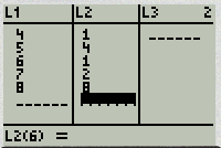
3. Enter the data values (one value per row) into L1. For any negative values you need to use the (-) key, not the subtraction key. Continue until all data is entered into L1. Enter the frequency value into L2.
4. Press the “STAT” key again
5. Use the arrow key to scroll over to “CALC”.
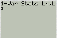
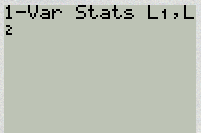
6. Select option 1: “1-Var Stats”
7. Indicate that the data is in L1,L2 (2nd, then 1 for L1, The comma is located above the 7 on the calculator, 2nd, then 2 for L2.) Or List: L1, FreqList L2 if using a newer calculator.
8. Scroll down to “Calculate” and hit “Enter”
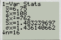
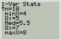
The summary statistics should now be displayed. Using “1-Var Stats” you can get the sample mean, sample standard deviation (Sx), population standard deviation, and 5 number summary.
 or
or 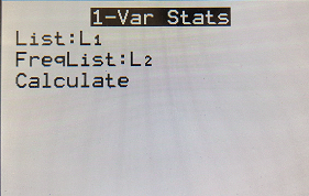
Quartiles, Five Number Summary, and Boxplots
The final measure of variability we must consider are the quartiles. Whereas the standard deviation was a measure of spread based around the mean, the quartiles are a measure of spread based around the median.
| Quartiles |
|
Quartiles are values that divide the data into quarters. The first quartile (Q1) is the value so that 25% of the data values are below it; the third quartile (Q3) is the value so that 75% of the data values are below it. You may have guessed that the second quartile (Q2) is the same as the median, since the median is the value so that 50% of the data values are below it. This divides the data into quarters; 25% of the data is between the minimum and Q1, 25% is between Q1 and Q2 (the median), 25% is between Q2 and Q3, and 25% is between Q3 and the maximum value. |
While quartiles are not a 1-number summary of variation like the range, the quartiles are used with the median, minimum, and maximum values to form a 5 number summary of the data.
| Five Number Theory |
|
The five number summary takes this form: Minimum, Q1, Median (Q2), Q3, Maximum |
To find the first quartile, we need to find the data value so that 25% of the data is below it. If n is the number of data values, we compute a locator by finding 25% of n. If this locator is a decimal value, we round up, and find the data value in that position. If the locator is a whole number, we find the mean of the data value in that position and the next data value. This is identical to the process we used to find the median, except we use 25% of the data values rather than half the data values as the locator.
| Example 4 |
|
Suppose we have measured 9 females and their heights (in inches), sorted from smallest to largest are: 59 60 64 65 66 67 68 70 72. Give the five-number summary for this data set. The 5-number summary gives the minimum value, Q1, Q2 (the median), Q3, and the maximum value. For this sample, the minimum value is 59, and the maximum is 72. To find the second quartile, find the median. 59 60 64 65 [66] 67 68 70 72 Q2 = 66 inches To find the first quartile, find the median of the data values less than Q2. 59 [60 64] 65 66 67 68 70 72 Q1 = 62 inches To find the third quartile, find the median of the data values above Q2. 59 60 64 65 66 67 [68 70] 72 Q3 = 69 inches The 5 number summary is: 59, 62, 66, 69, 72. |
| Example 5 |
|
Suppose we had measured 8 females and their heights (in inches), sorted from smallest to largest are: 59 60 62 64 66 67 69 70 Give the five-number summary for this data set. For this sample, the minimum value is 59, and the maximum is 70. To find the second quartile, find the median. 59 60 62 [64 66] 67 69 70 Q2 = 65 inches To find the first quartile, find the median of the data values less than Q2. 59 [60 62] 64 66 67 69 70 Q1 = 61 inches The third quartile, find the median of the data values above Q2. 59 60 62 64 66 [67 69] 70 Q3 = 68 inches The 5 number summary for this data set would be: 59, 61, 65, 68, 70. |
| Example 6 | ||||||||||
|
Returning to our quiz score data. In each case, the first quartile locator is 0.25(10) = 2.5, so the first quartile will be the 3rd data value, and the third quartile will be the 8th data value. Creating the five-number summaries:
|
Of course, with a relatively small data set, finding a five-number summary is a bit silly, since the summary contains almost as many values as the original data.
| You Try 3.4.C | ||||||||||||||||||||||||||||||||||||
The total cost of textbooks for the term was collected from 36 students. Find the 5 number summary of this data:
|
Note that the 5 number summary divides the data into four intervals, each of which will contain about 25% of the data.
It is often difficult to picture how the 5 number summary shows the variability in a data set. For visualizing data, there is a graphical representation of the 5-number summary called a box plot, or box and whisker graph.
| Boxplot (Box and Whisper Plot) |
|
A boxplot is a graphical representation of a five-number summary. To create a box plot, a number line is first drawn. A box is drawn from the first quartile to the third quartile, and a line is drawn through the box at the median. “Whiskers” are extended out to the minimum and maximum values. |
NOTE: It is important to use consistent intervals of values on the number line in a boxplot. For example, if you start your number line at 0, you may want to make tick marks at 10, 20, 30, etc. You should never use different intervals on the same axis. For example, do not have your first tick mark at 10, your next at 15, then the next at 35, etc. This will counteract the entire purpose of a boxplot, which is to see how the spread differs within the data set.
| Example 7 |
|
The box plot below is based on the 9 female height data with 5 number summary: 59, 62, 66, 69, 72.
|
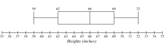
Notice that the horizontal axis used consistently spaced units (increments of 1).
| Example 8 |
|
The box plot below is based on the household income data with 5 number summary: 15, 27.5, 35, 40, 50
|
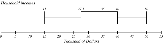
Notice that the horizontal axis used consistently spaced units (increments of 5).
| You Try S.4.D |
|
Create a boxplot based on the textbook price data from the last You Try problem 3.4C. |
Box plots are particularly useful for comparing data from two populations.
| Example 9 |
|
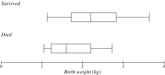
The boxplot below is based on the birth weights of infants with severe idiopathic respiratory distress syndrome (SIRDS). The boxplot is separated to show the birth weights of infants who survived and those that did not.
Comparing the two groups, the boxplot reveals that the birth weights of the infants that died appear to be, overall, smaller than the weights of infants that survived. In fact, we can see that the median birth weight of infants that survived is the same as the third quartile of the infants that died. Similarly, we can see that the first quartile of the survivors is larger than the median weight of those that died, meaning that over 75% of the survivors had a birth weight larger than the median birth weight of those that died. Looking at the maximum value for those that died and the third quartile of the survivors, we can see that over 25% of the survivors had birth weights higher than the heaviest infant that died. The box plot gives us a quick, albeit informal, way to determine that birth weight is quite likely linked to survival of infants with SIRDS. |
| Example 10 |
|
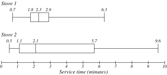
The box plot of service times for two fast-food restaurants is shown below.
While store 2 had a slightly shorter median service time (2.1 minutes vs. 2.3 minutes), store 2 is less consistent, with a wider spread of the data. At store 1, 75% of customers were served within 2.9 minutes, while at store 2, 75% of customers were served within 5.7 minutes. Which store should you go to in a hurry? That depends upon your opinions about luck – 25% of customers at store 2 had to wait between 5.7 and 9.6 minutes. |
| Percentiles |
Percentiles are used in statistics to indicate a value below which a certain percentage of the data values fall. For example, if you score in the 60th percentile on a standardized test, it means that 60% of the other scores were lower than yours, (and 40% were higher).
| Example 11 |
|
a. What percentage of the values in a data set lie at or below the 30th percentile? b. What percentage of the values in a data set lie at or above the 30th percentile? c. If 500 measurements were taken, approximately how many would be at or below the 30th percentile? d. If 500 measurements were taken, approximately how many would be at or above the 30th percentile? |
|
a. By definition, 30% of the data values lie at or below the 30th percentile. b. Since 30% lie below the 30th percentile, 100% - 30% = 70% of the data values lie above it. c. 30% of 500 = .30(500) = 150 values lie below the 30th percentile d. 70% of 500 = .70(500) = 350 values lie above the 30th percentile. |
In general, for any set of numerical data, 50% of the data values are below the median, so the median will always represent the 50th percentile. The lower quartile (Q1) would be the 25th percentile, and the upper quartile (Q3) would be the 75th percentile.
| Example 12 |
|
In example 5 we looked at the heights (in inches), of a sample of 8 females. The heights were: 59, 60, 62, 64, 66, 67, 69, 70, and we found the 5 number summary to be: 59, 61, 65, 68, 70. a. What is the 25th percentile of the heights of females? b. What is the 75th percentile of the heights of females? |
|
a. We know that the 25th percentile is the height such that 25% of heights are lower, and 75% of heights are higher. This is the same as the first quartile. The 25th percentile is 61 inches. b. We know that the 75th percentile is the height such that 75% of heights are lower, and 25% of heights are higher. This is the same as the third quartile. The 75th percentile is 68 inches. |
In this text, we only examine the process of finding the 25th, 50th, and 75th percentiles. Using other statistical techniques, it is possible to find the data value corresponding to any percentile in the data set.
| Calculator Instructions for Finding Summary Statistics Using TI-83/84 |
1. Turn on the calculator
2. Press the “STAT” key
3. Hit “Enter” on option 1: “Edit”
This will bring you to a screen that contains lists: L1, L2, L3, etc.
3. Enter the data values (one value per row) into L1. For any negative values you need to use the (-) key, not the subtraction key. Continue until all data is entered into L1.
4. Press the “STAT” key again
5. Use the arrow key to scroll over to “CALC”.
6. Select option 1: “1-Var Stats”
7. Indicate that the data is in L1
8. Scroll down to “Calculate” and hit “Enter”
The summary statistics should now be displayed. You may scroll down with your arrow key to get remaining statistics. Using “1-Var Stats” you can get the sample mean, sample standard deviation, population standard deviation, and 5 number summary.
| Example 13 |
|
Suppose we had measured 8 females and their heights (in inches), sorted from smallest to largest are: 59 60 62 64 66 67 69 70 Give the five-number summary for this data set.
The 5 number summary for this data set would be: 59, 61, 65, 68, 70. |
| Example 14 |
|
Find the 5 number summary for the bar graph.
4 5 5 5 5 6 7 7 8 8 Minimum Value = 4 First Quartile = 5 Second Quartile = 5.5 Third Quartile = 7 Maximum Value = 8 The 5 number summary is: 4, 5, 5.5, 7, 8
|

References
[11] The reason we do this is highly technical, but we can see how it might be useful by considering the case of a small sample from a population that contains an outlier, which would increase the average deviation: the outlier very likely won't be included in the sample, so the mean deviation of the sample would underestimate the mean deviation of the population; thus we divide by a slightly smaller number to get a slightly bigger average deviation.
Section S.4 Answers to You Try Problems
S.4.A
The range of the data is $0.70.
S.4.B
The standard deviation of the data is $0.26.
S.4.C
The data is already in order, so we don’t need to sort it first.
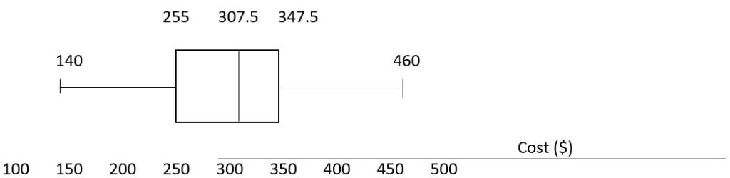
The minimum value is $140 and the maximum is $460.
There are 36 data values so n = 36. n/2 = 18, which is a whole number, so the median is the mean of the 18th and 19th data values, $305 and $310. The median is $307.50.
To find the first quartile, we calculate the locator, L = 0.25(36) = 9. Since this is a whole number, we know Q1 is the mean of the 9th and 10th data values, $250 and $260. Q1 = $255.
To find the third quartile, we calculate the locator, L = 0.75(36) = 27. Since this is a whole number, we know Q3 is the mean of the 27th and 28th data values, $345 and $350. Q3 = $347.50.
The 5 number summary of this data is: $140, $255, $307.50, $347.50, $460
S.4.D