
Section S.6 - Standard Scores (z-scores), Finding Percentages with Normally Distributed Variables
Standard Scores (z-scores)
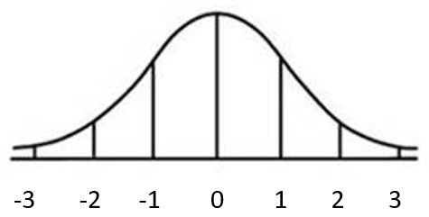
The Empirical Rule only applies when a value is exactly 1, 2, or 3 standard deviations away from the mean. This is not usually the case.
A standard score (also called “z-score”) is the number of standard deviations a data value is from the mean of the distribution. We can plot z-scores on a special normal distribution called the standard normal distribution. The standard normal distribution is a normal distribution that always has population mean 0 and population standard deviation of 1.
| Standard Scores (z-scores) |
|
A standard score (also called “z-score”) is the number of standard deviations a specific data value is from the mean of the distribution. Standard scores (often abbreviated by the letter z) have the following characteristics:
To calculate the z-score for any data value, x, use the following formula: z = [latex]\frac{x~-~mean}{standard~-~deviation}[/latex] |
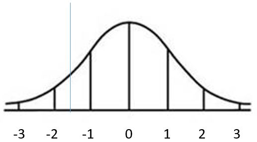
Applying the Empirical Rule to the standard normal distribution, we know that 68% of all z-scores will be between -1 and 1, 95% of all z-scores will be between -2 and 2, and 99.7% of all z-scores will be between -3 and 3. A z-score below -3 or above 3 is possible, but is very unlikely.
| Example 1 |
|
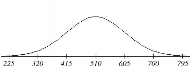
Scores on a standardized test were normally distributed with a mean of 510 and a standard deviation of 95. a. A student scores 365 points on the test. What is his standard score? b. What test score corresponds to a standard score of 2.2? |
|
a. Here, x = 365, mean = 510, and standard deviation = 95.
So we have: z = [latex]\frac{365~-~510}{95}[/latex] = [latex]\frac{-145}{95}[/latex] ≈ -1.53 So this student’s score was about 1.53 standard deviations below the mean. The student’s standard score is 1.53. You can see visually that the test score of 365 corresponds exactly to the z-score of -1.53 on the standard normal distribution curve below.
b. Here, z = 2.2, mean = 510, and standard deviation = 95.
We are solving for x. 2.2 = [latex]\frac{x~-~510}{95}[/latex] (Multiply both sides by 95) 209 = x - 510 790 = x
So a test score of 719 corresponds to a standard score of 2.2. |

| Example 2 |
|
The weights of a certain dog breed are approximately normally distributed with a mean of 62 pounds, and a standard deviation of 6 pounds. a. A dog of this breed weighs 55 pounds. What is the dog’s z-score? Is this dog’s weight unusual for this breed? b. A dog has a z-score of -3.2. What is the dog’s weight? |
|
a. Here, x = 55, mean = 62, and standard deviation = 6. So we have: z = [latex]\frac{55~-~62}{6}[/latex] = [latex]\frac{-7}{6}[/latex] ≈ -1.17 So this dog’s weight was about 1.17 standard deviations below the mean. No, the dog’s weight is well within 3 standard deviations of the mean, so it is not unusual. b. Here, z = -3.2, mean = 62, and standard deviation = 6. We are solving for x. -3.2 = [latex]\frac{x~-~62}{6}[/latex] -19.2 = x - 62 42.8 = x So a z-score of -3.2 corresponds to a dog that weighs 42.8 pounds. Since this z-score is less than -3, this is an unusually low z-score. This indicates that this dog’s weight is unusually low. |
| You Try S.6.A |
|
The lengths of mature trout in a local lake are approximately normally distributed with a mean of 13.2 inches, and a standard deviation of 1.8 inches. a. Draw and label the distribution of trout length. b. Draw and label the standard normal distribution. c. Find the z-score corresponding to a fish that is 19 inches long. d. How long is a fish that has a z-score of -0.85? e. Draw the z-score from part c on your graph from part b. |
Now we know how to convert any value of a variable that is approximately normally distributed into a z-score. This z-score represents a location on the standard normal distribution. You may be thinking, ok, so I can convert an observed value of a variable into a z-score, but why is that useful? In the next section we will begin to answer this question.
Finding Percentages with Normally Distributed Variables
We will start out this section with a question: Why go to the trouble of calculating the z-score that corresponds to an observed value? We will answer this question through the use of the following examples:
| Example 3 |
|
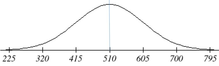
Consider the data set consisting of scores on a standardized test. The test scores were normally distributed with a mean of 510 and a standard deviation of 95. What percentage of students scored less than 510 on the test? |
|
We can answer this question using what we already know about normal distributions. Specifically, they are centered about their mean, and symmetric about their mean. If we draw a line to divide the data set at the mean, it is clear that the percentage of observations that are less than the mean should be 50% (with another 50% being greater than the mean).
We could answer this question just using properties of normal distributions. |
| Example 4 (Part I) |
|
Consider again the data set consisting of scores on a standardized test were normally distributed with a mean of 510 and a standard deviation of 95. What percentage of students scored less than 650 on the test? |
|
This is the same question we just answered, but you can see quickly that changing the observed value from 510 to 650 made this question much more difficult to answer. We don’t know the exact percentage of scores that are less than 650. If we had a list of all of the test scores, we could count how many of them were below 650. We could then divide by the total number of scores, and convert to a percentage. That sounds simple enough, but we don’t have the list of test scores. So how can we answer this question knowing just the shape of the distribution, the mean, and the standard deviation? We will come back to this example and answer this question. |
At this point, in order to continue solving the problem above, we have to know how the find the percentage of values (areas) under the normal distribution curve with mean 510 and standard deviation 95. That involves complex formulas and calculus. To avoid those requirements, we will use the standard normal distribution curve. Because we learned in the last section how to convert any normally distributed variable into the standard normal, all we need to know are percentages (or areas) under the standard normal distribution curve. These values can be readily looked up using a z-table, or can be found using your graphing calculator.
The following z-table provides areas (percentages of values) under the standard normal curve that lie to the left of specified z-scores. This type of table is called a Cumulative Z-Score Table.
| Abbreviated Table of Areas under the Standard Normal Curve |
|
Note: All values are the area to the LEFT of the specified z-score. Area to the Right = 1 – Area to the Left |
|
Z-Score |
Area |
Z-Score |
Area |
Z-Score |
Area |
Z-Score |
Area |
|
-4.0 |
0.00003 |
-1.0 |
0.1587 |
0.0 |
0.5000 |
1.1 |
0.8643 |
|
-3.5 |
0.0002 |
-0.95 |
0.1711 |
0.05 |
0.5199 |
1.2 |
0.8849 |
|
-3.0 |
0.0013 |
-0.90 |
0.1841 |
0.10 |
0.5398 |
1.3 |
0.9032 |
|
-2.9 |
0.0019 |
-0.85 |
0.1977 |
0.15 |
0.5596 |
1.4 |
0.9192 |
|
-2.8 |
0.0026 |
-0.80 |
0.2119 |
0.20 |
0.5793 |
1.5 |
0.9332 |
|
-2.7 |
0.0035 |
-0.75 |
0.2266 |
0.25 |
0.5987 |
1.6 |
0.9452 |
|
-2.6 |
0.0047 |
-0.70 |
0.2420 |
0.30 |
0.6179 |
1.7 |
0.9554 |
|
-2.5 |
0.0062 |
-0.65 |
0.2578 |
0.35 |
0.6368 |
1.8 |
0.9641 |
|
-2.4 |
0.0082 |
-0.60 |
0.2743 |
0.40 |
0.6554 |
1.9 |
0.9713 |
|
-2.3 |
0.0107 |
-0.55 |
0.2912 |
0.45 |
0.6736 |
2.0 |
0.9772 |
|
-2.2 |
0.0139 |
-0.50 |
0.3085 |
0.50 |
0.6915 |
2.1 |
0.9821 |
|
-2.1 |
0.0179 |
-0.45 |
0.3264 |
0.55 |
0.7088 |
2.2 |
0.9861 |
|
-2.0 |
0.0228 |
-0.40 |
0.3446 |
0.60 |
0.7257 |
2.3 |
0.9893 |
|
-1.9 |
0.0287 |
-0.35 |
0.3632 |
0.65 |
0.7422 |
2.4 |
0.9918 |
|
-1.8 |
0.0359 |
-0.30 |
0.3821 |
0.70 |
0.7580 |
2.5 |
0.9938 |
|
-1.7 |
0.0446 |
-0.25 |
0.4013 |
0.75 |
0.7734 |
2.6 |
0.9953 |
|
-1.6 |
0.0548 |
-0.20 |
0.4207 |
0.80 |
0.7881 |
2.7 |
0.9965 |
|
-1.5 |
0.0668 |
-0.15 |
0.4404 |
0.85 |
0.8023 |
2.8 |
0.9974 |
|
-1.4 |
0.0808 |
-0.10 |
0.4602 |
0.90 |
0.8159 |
2.9 |
0.9981 |
|
-1.3 |
0.0968 |
-0.05 |
0.4801 |
0.95 |
0.8289 |
3.0 |
0.9987 |
|
-1.2 |
0.1151 |
0.0 |
.5000 |
1.0 |
0.8413 |
3.5 |
0.9998 |
|
-1.1 |
0.1357 |
|
|
|
|
4.0 |
0.99997 |
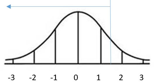
| Finding Areas to the Left of Z-Scores |
| Example 4 (Part II) |
|
Let’s go back to the previous example, using what we now know about finding percentages under the standard normal distribution curve. Our data consisted of scores on a standardized test that were normally distributed with a mean of 510 and a standard deviation of 95. We wanted to know what percentage of students scored less than 650 on the test. |
|
As starting point, we will calculate the z-score that corresponds to a test score of 650. z = [latex]\frac{650~-~540}{95}[/latex] = [latex]\frac{140}{95}[/latex] = 1.47 This tells us that the percentage of students who score less than 650 on the test will be equal to the percentage of observations that are less than 1.47 under the standard normal curve.
Using the z-table: Look in the z-score columns to find the integer and first decimal in your z-score. For this example, we will round 1.47 to 1.5. The area from the table is .9332. We can say that approximately 93.32% of all test scores were less than 650. |
| Example 5 |
|
The weights of a certain dog breed are approximately normally distributed with a mean of 62 pounds, and a standard deviation of 6 pounds. Find the percentage of dogs of this breed that weigh less than 55 pounds. |
|
We need to start out by finding the z-score that corresponds to a dog weighing 55 pounds. z = [latex]\frac{55~-~62}{6}[/latex] = [latex]\frac{-7}{6}[/latex] = -1.17
Using the Table: In the z-table, we don’t have -1.17. The closest value to -1.17 is -1.2. Our answer will be an approximation. The corresponding area to the left is 0.1151. The percentage of dogs of this breed that weight less than 55 pounds is approximately 11.51%. |
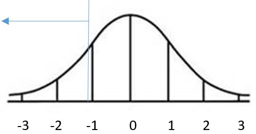
| Finding Areas to the Right of Z-Scores |
| Example 6 |
|
The weights of a certain dog breed are approximately normally distributed with a mean of 62 pounds, and a standard deviation of 6 pounds. Find the percentage of dogs of this breed that weigh MORE than 55 pounds. |
|
We need to start out by finding the z-score that corresponds to a dog weighing 55 pounds. z = [latex]\frac{55~-~62}{6}[/latex] = [latex]\frac{-7}{6}[/latex] = -1.17 This time we need to find the percentage of z-scores that are greater than -1.17 (or to the right of -1.17).
Using the Table: In the z-table, we don’t have -1.17. The closest value to -1.17 is -1.2. Our answer will be an approximation. The corresponding area to the left is 0.1151. Use subtraction to find the area the right, 1 - 0.1151 = 0.8849. The percentage of dogs of this breed that weight more than 55 pounds is approximately 88.49%. |
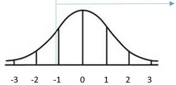
The previous example illustrates an important property about areas under the standard normal distribution. Since the total percentage of values under the distribution curve is always equal to 100% (or 1) the area to the left of a z-score plus the area to the right of that same z-score will always equal 1 (or 100% of the observations).
| You Try 3.6.B |
|
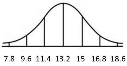
The annual rainfall in a certain region is approximately normally distributed with mean 33.5 inches and standard deviation 5.6 inches. a. What percentage of years will have an annual rainfall of less than 30 inches? b. What percentage of years will have an annual rainfall of more than 40 inches? |
| Finding the Area Between Two Z-Scores |
Recall that in Section 3.5 we learned the Empirical Rule (or 68-95-99.7 Rule). This rule allowed us to find the percentage of observations that lied between specific values of our variable. While this is useful, there are many occasions where the data values we are interested in do not happen to fall right at 1, 2, or 3 standard deviations away from the mean.
|
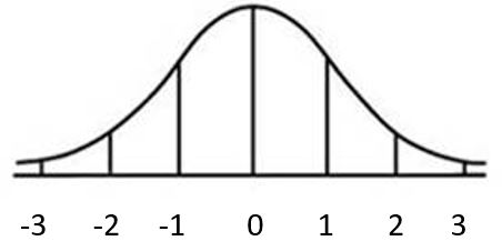
We know from the Empirical Rule that about 68% of all observations will fall between -1σ and 1σ
(between -1 and 1 in the standard normal distribution) |
|
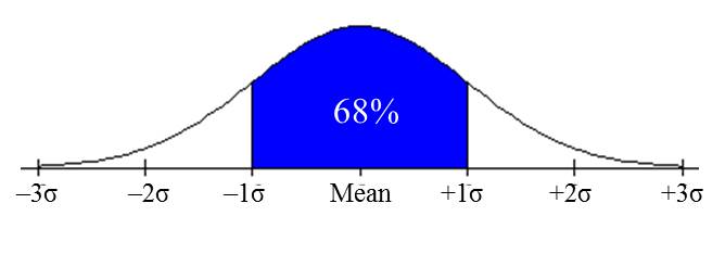
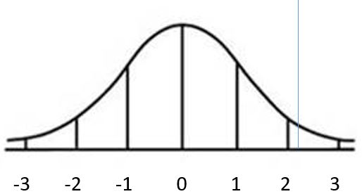
What if we wanted to find the percentage of all observations that will have z-scores between -2 and 2? Again, using the Empirical Rule, we know the answer is approximately 95%.
What if we wanted to find the percentage of all observations that will have z-scores between -1.5 and 1.5? This becomes much more challenging. We would expect the answer to be between 68% and 95%, but we can now get much more precise.
| Example 7 |
|
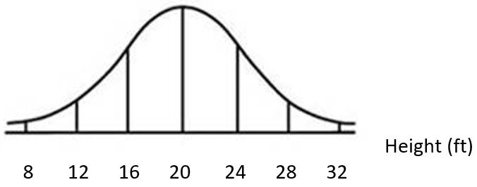
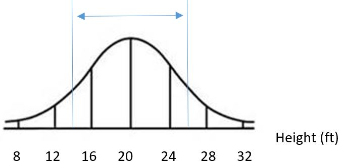
A scientist finds that the heights of a certain tree are approximately normally distributed with mean 20 feet and standard deviation 4 feet. The associated normal distribution curve is as follows:
Suppose we are asked to find the percentage of all such trees that are between 14 and 26 feet tall. The percentage of trees that are between 14 and 26 feet tall corresponds to the percentage of values that are between the two lines drawn on the curve below:
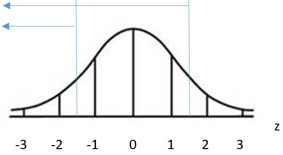
We can find the associated z-scores that correspond to tree heights of 14 ft. and 26 ft. using the z-score formula from the previous section: z = [latex]\frac{14~-~20}{4}[/latex] = [latex]\frac{26~-~20}{4}[/latex] = -1.5 and z = [latex]\frac{26~-~-20}{4}[/latex] = [latex]\frac{6}{4}[/latex] = 1.5 We now know that the percentage of trees between 14 and 26 feet tall is the same as the percentage of observations between -1.5 and 1.5 under the standard normal distribution.
Using the table, the area that we are looking for is the area BETWEEN -1.5 and 1.5. If we subtract the area to the left of -1.5 from the area to the left of 1.5, our answer will be just the remaining area between the two z-scores. Area to the left of -1.5 = 0.0668 Area to the left of 1.5 = 0.9332 Area in between -1.5 and 1.5 = 0.9332 – 0.0668 = 0.8664. Therefore, 86.64% of trees are between 14 and 26 feet tall. |
| You Try S.6.C |
|
The annual rainfall in a certain region is approximately normally distributed with mean 33.5 inches and standard deviation 5.6 inches. What percentage of years will have an annual rainfall of between 30 and 40 inches? |
Section S.6 Answers to You Try Problems
S.6.A.
a.
b.
c. z = 3.22
d. 11.67 inches
e.
S.6.B
a. z = -0.63. Area to the left of -0.63 is 0.2578, or 25.78%
b. z = 1.16. Area to the right of 1.16 is 0.1151, or 11.51%
S.6.C
0.8849 - 0.2578 = .6271.
In this region, 62.71% of all years will have annual rainfall between 30 and 40 inches.
