8.5 – Hypothesis Testing Steps

Now that we have covered some of the basic concepts of null hypothesis significance testing (NHST), we are going to organize it into a series of steps that we will follow each time we test a research hypothesis. Here are the steps:

1. State Hypotheses to Test
2. Establish the Criterion for a Decision
3. Collect and Graph Data
4. Compute the Test Statistic
5. Make a Statistical Decision
6. Share the Results

1. State Hypotheses to Test

The first step of null hypothesis significance testing (NHST) is to state the hypotheses that we intend to test. We actually state two hypotheses: the null hypothesis (H₀) and the alternative hypothesis (H₁). However, as the name, “null hypothesis significance testing,” indicates we are ultimately going to test only the null hypothesis.

As discussed in the previous section, we are going to state our hypotheses in sentence and symbol form. The sentence form typically makes more sense intuitively, so it’s good to start there. However, the symbol form version is particularly important for hypothesis testing because it will often help specify some components of our statistical formulas.

2. Establish the Criterion for a Decision

Once we have stated the null hypothesis, which is a prediction of a lack of treatment effect or relationship, we will need to determine what research results would make us question whether the null hypothesis is the best explanation for the results of our study. To do this, we would think about what kinds of results we would expect to get if the null hypothesis were true and what kinds of results we would be less likely to expect to get if the null hypothesis were true. Then, we determine a cut-off point where we are comfortable saying that any research result short of this cut-off point is consistent with the null hypothesis, and any result equal to or greater than the cut-off point is not consistent with the null hypothesis. Essentially, we will “draw a line in the sand” and then see if our research results cross that line.

In setting this criterion, we will use probability. Specifically, we are going to specify what is called the significance level, or the “alpha level,” depicted by α (the Greek letter, “alpha”), which is the probability of rejecting the null hypothesis, H₀, if the null hypothesis is true (H₀ = true). In other words, it is the probability of claiming that there is an effect, difference, or correlation when there actually isn’t one.

Conventionally, α is usually set at 0.05 or 0.01, with 0.05 being the most common. This will also, for the most part, be the case for examples in this textbook.

When α = 0.05, we are setting our criterion or cut offcritical region at the point at which there is a probability of 0.05, or 5% chance, of rejecting the null when the null is true.

Once the alpha level is selected, it can then be used to determine the critical value of the test statistic and thus the cutoff point for the critical region (also known as the “region of rejection“). This critical value or values (depending on whether you are doing a one-tailed test or two-tailed test) are the “lines in the sand” that we have determined are the point at which the result would no longer be considered consistent with the null hypothesis and would lead us to think that the null hypothesis is “probably wrong.”

As an example, let’s say that researchers wanted to explore whether sleep deprivation impacts short-term memory. Specifically, they believe that sleep deprivation will impair short-term memory. To test their hypothesis, they design a research study. They invite 100 people to their lab to spend the night. Participants are woken up every hour throughout the night. Then in the morning, they are asked to complete the Saenz Short-Term Memory Test (SSTMT), which under normal circumstances is normally distributed and has a mean of μ = 50 and a standard deviation of σ = 10.

Because the scientific method requires researchers to test the null hypothesis, we can then explore what it would look like if these 100 people were to take the SSTMT without any impairment. Because the SSTMT is normally distributed and has a mean of μ = 50 and a standard deviation of σ = 10, we can use the Central Limit Theorem to predict all the possible sample means for samples of 100 people.

The Central Limit Theory will predict the following about these sample means:

1. They will form a roughly normal, or bell-shaped, distribution.
2. The mean of all these SSTMT sample means will be roughly the same as the population mean of the SSTMT (μ = 50).
3. The standard deviation of these sample means can be calculated as the standard error, equal to: A statistic that examines research data to test hypotheses in null hypothesis significance testing (NHST).

Thus, we can create a graph of the distribution of all of the possible sample means as follows:

Remember that this distribution of sample means depicts all of the possible sample means we could get from samples of 100 people who were given the SSTMT without any treatment effect. We expect most people to score around 50 on the SSTMT because that is the average score. However, we will also have people score above or below the mean because of their relatively poor or good memory skills. Thus, if we think of this graph as a distribution of thousands of sample means, it would look like this:

Now that we can visualize all of the possible sample means that we could get if there is no treatment effect (the null hypothesis is true; in other words, H₀: μ_{sleep deprivation} = 50), we can use that distribution to “draw a line in the sand” that delineates where we start to get sample means that really make us question whether the null hypothesis is actually true.

Sample means near 50 are consistent with the null hypothesis because that is exactly what we would predict a sample mean would likely be if there were no treatment effect. Why? Think of it this way. We know that people normally score around 50 on the SSTMT (we are told this when we are told that the SSTMT has a population mean of μ = 50). Then, if we took a sample of n = 100 people and gave them the SSTMT without doing anything to them (in other words, no treatment effect), we would expect the mean of those 100 people to be pretty close to 50 on the test.

On the other hand, if we get a sample mean that is far away from 50, that would start to make us wonder if something weird is going on. By now, hopefully, we know that sampling error exists, so we should not expect all our sample means to be exactly 50. Sample means will differ somewhat from 50 in either direction because of sampling error.

Yet, by calculating the standard error (σ_M), we actually know the average amount of sampling error that we can expect. Based on our calculation of standard error with a sample of 100 individuals, we can expect about 1 point of sampling error. In other words, our sample means should be right around 50, plus or minus about 1 point on average. That is what the graphs above depict.

Then, with that knowledge, we can use probability and our alpha (α) to “draw our line in the sand” and designate our critical region or regions. This would allow us to determine the point at which a sample mean of people who received our treatment would be so unusual that we would decide that it was very unlikely that the treatment didn’t have an effect. Setting the alpha level will determine exactly how “unlikely.”

Let’s say the researchers use an alpha level of α = 0.05. This means that they only want a 5% chance (probability of 0.05) that they would reject the null hypothesis (claim an effect, difference, or correlation) when the null hypothesis is actually true (there is no effect, difference, or correlation).

This 5% (0.05 probability) can then be applied to the distribution of sample means. Specifically, we will determine the 5% of the distribution of sample means that is the most inconsistent with the null hypothesis and thus most consistent with the alternative hypothesis.

There are two ways this can be done:

• Directional Hypothesis, or “One-Tailed” Hypothesis
• Non-Directional Hypothesis, or “Two-Tailed” Hypothesis

We will explore directional hypotheses first because they tend to be the most consistent with common sense. However, non-directional hypotheses are more common because they are considered to be a little more conservative and more appropriate for most situations.

Directional or One-Tailed Hypotheses

Directional hypothesis tests specify the “direction” that the researchers predict the results would go if there is an effect, difference, or correlation. For example, the researchers exploring the impact of sleep deprivation on memory would likely predict that sleep deprivation would lower memory scores. In other words, they would predict that the direction of the effect would be a negative effect.

The hypotheses in this study would be:

• Alternative: Sleep Deprivation will reduce memory.
• Null: Sleep deprivation will not reduce memory.

Or, in symbols:

• H₁: μ_{sleep deprivation} < 50
• H₀: μ_{sleep deprivation} ≥ 50

Then, if we combine an alpha of α = 0.05 and non-directional hypotheses, we can look at the distribution of sample means and identify the 5% of the distribution that is inconsistent with the null hypothesis and thus consistent with the alternative hypothesis.

Using the null hypothesis, we would conclude that sample means near 50 or higher than 50 are consistent. However, sample means less than 50 are not as consistent. But the question is, how much lower than 50? That’s where the alpha comes in. It would be the 5% extremely low sample means. Thus, we get the following:

In this distribution, we have shaded the 5% of sample means that are unusually low. The sample means in this shaded area are inconsistent with the null hypothesis (that sleep deprivation will not reduce memory) and instead are more consistent with the alternative hypothesis (that sleep deprivation will reduce memory).

As you can see, we have shaded only one tail of the distribution. That is why directional hypotheses are called “one-tailed” hypotheses.

Technically, what we have just shaded is called the critical region. It is the region of the distribution where the researcher would start to question the null hypothesis.

We can then use the critical region to “draw a line in the sand,” where that line is the cut-off point at which a sample mean is now in the critical region. To do this, we will simply use the techniques we learned in the previous two chapters to determine a cut-off point for a distribution percentage.

Looking at the distribution of sample means above, we can see that the shaded area is a “tail.” We then need to convert our percentage to a proportion. To convert our percentage of 5% to a proportion, we simply divide it by 100. Thus, we look for the proportion of 0.0500 (make sure to use four decimal places because the proportions in our Unit Normal Table go to four decimal places).

As you can see in the table, the exact proportion of 0.0500 does not exist in the Tail column. The two closest proportions to 0.0500 are 0.0505 and 0.0495. Typically, we would then pick the proportion that is the closest to our proportion. By subtracting each of the proportions in the table from our proportion of 0.0500 we find that both 0.0505 and 0.0495 are exactly 0.0005 or 5 ten-thousandths away:

0.0505 – 0.0500 = 0.0005
0.0500 – 0.0495 = 0.0005

As stated in Chapter 6, when a situation like this happens and the target proportion is equidistant from two proportions in the Unit Normal Table, we will choose the higher of the two z-scores. At the time, we indicated that the reason for this would make more sense in the future and has to do with being careful to not exceed a specified probability when we are using hypothesis testing and inferential statistics. And now is the time to explain that.

When we set an alpha level of α = 0.05, we are declaring that we only want a 0.05 probability, or 5% chance, that we might make a Type I error (when we claim an effect, difference, or correlation when, in reality, there isn’t one). If we follow our rule that when a target proportion is equidistant from two proportions in the Unit Normal Table and choose the higher z-score, in this case, z = 1.65, we would technically have a tail of exactly 0.0495, or 4.95%, which is a bit smaller than we wanted. If, on the other hand, we choose the lower z-score,  z = 1.64, we would technically have a tail of exactly 0.0505, or 5.05%, which is a bit larger than we wanted, and this is where we will have a problem in terms of using inferential statistics. With an alpha level of α = 0.05, we are essentially declaring that we want no more than a 0.05 probability, or 5% chance, that we might make a Type I error. Thus, using the z-score cutoff of 1.64 would violate that, and thus we use the higher z-score of z = 1.65.

Be careful, though, because there is one last step that can be critically important. We should now return to our distribution of sample means to label the “line in the sand” for our critical region. Technically, this is called a critical value. To do this, however, we need to:

1. Add a second axis below the axis for the Sample Means (M)
2. Draw a tick mark (or tick marks in the case of two-tailed tests) at the critical region cutoff
3. Label the tick mark (or tick marks) with the appropriate z-score(s) that we just found in the Unit Normal Table for the appropriate alpha level.
4. Make sure that the sign (“+” or “-“) is correct. Z-scores to the left of the mean are negative. Z-scores to the right of the mean are positive.

Because our critical region is to the left of the mean, the z-score cutoff should be -1.65.

We have now drawn a “line in the sand” indicating the point at which we will officially think that a statistical result is too weird to happen if the null is true. This cutoff point is called the critical value and is often depicted as:

z_critical = -1.65

The word “critical” in the subscript is an indication that this is the critical value of the z-score that determines our critical region. It is abbreviated as “z_crit” in some places.

Now that we’ve drawn the “line in the sand” and determined exactly how extreme of a result we would need before we would question the null hypothesis, we are ready to run our study and see if sleep deprivation leads to a memory score that is extremely low enough that we would question the hypothesis that sleep deprivation will not reduce memory scores (the null hypothesis).

Non-Directional or Two-Tailed Hypotheses

Unlike directional hypotheses, non-directional hypotheses do not specify a direction but are instead interested in detecting impacts in either direction. Using the example of the research on sleep deprivation and memory, a non-directional hypothesis test would predict that sleep deprivation would impact memory in any direction. In other words, they would predict that the effect could either be positive or negative.

The hypotheses in this study would be:

• Alternative: Sleep Deprivation will affect memory.
• Null: Sleep deprivation will not affect memory.

Or, in symbols:

• H₁: μ_{sleep deprivation} ≠ 50
• H₀: μ_{sleep deprivation} = 50

Then, if we combine an alpha of α = 0.05 and non-directional hypotheses, we can look at the distribution of sample means and identify the 5% of the distribution that is inconsistent with the null hypothesis and thus consistent with the alternative hypothesis.

Using the null hypothesis, we would conclude that sample means near 50 or higher than 50 are consistent. However, sample means that are either more or less than 50 are not as consistent. But the question is, how much lower or higher than 50? That’s where the alpha comes in. It would be the 5% extreme sample means (in either direction). Thus, we get the following:

In this distribution, we have shaded the 5% of sample means that are either low or extremely high. The sample means in this shaded area are inconsistent with the null hypothesis (that sleep deprivation will not affect memory) and instead are more consistent with the alternative hypothesis (that sleep deprivation will affect memory).

As you can see, we have shaded only two tails of the distribution. That is why directional hypotheses are called “two-tailed” hypotheses.

Because there are two tails, it is important to note that when using a two-tailed hypothesis our alpha level of α = 0.05 needs to be split in half to be distributed equally on both sides. Thus, each of the tails depicts 2.5% (half of 5%) of the entire distribution.

Technically, what we have just shaded is called the critical region. It is the region of the distribution where the researcher would start to question the null hypothesis.

We can then use the critical region to “draw lines in the sand” where those lines are the cut-off points at which a sample mean would be considered to be in the critical region. To do this, we will simply use the techniques we learned in the previous two chapters to determine the cut-off points for a distribution percentage.

Looking at the distribution of sample means above, we can see that the shaded areas are both “tails.” We then need to convert our percentage to a proportion. At this point, we can focus on the tail to the right. To convert our percentage of 2.5% to a proportion, we simply divide it by 100. Thus, we look for the proportion of 0.0250 (make sure to use four decimal places because the proportions in our Unit Normal Table go to four decimal places).

As you can see in the table, the exact proportion of 0.0250 does exist in the Tail column. Thus, we will use the corresponding z-score of 1.96 as our cutoff for the tail to the right. Because normal distributions are symmetrical, we also now know the z-score cutoff for the tail to the left; it will be -1.96.

We can now return to our distribution of sample means to label the “lines in the sand” for our critical regions, our critical values. To do this, however, we need to:

1. Add a second axis below the axis for the Sample Means (M)
2. Draw a tick mark (or tick marks in the case of two-tailed tests) at the critical region cutoff
3. Label the tick mark (or tick marks) with the appropriate z-score(s) that we just found in the Unit Normal Table for the appropriate alpha level.
4. Make sure that the sign (“+” or “-“) is correct. Z-scores to the left of the mean are negative. Z-scores to the right of the mean are positive.

We have now drawn the “lines in the sand” indicating the points at which we will officially think that a statistical result is too weird to happen if the null is true. These cutoff points are called the critical values and are depicted as:

z_critical = ±1.96

It can be helpful to remember that non-directional, or two-tailed, hypotheses will always have two critical values and will use the “plus/minus” sign (±).

Now that we’ve drawn the “lines in the sand” and determined exactly how extreme of a result we would need before we would question the null hypothesis, we are ready to run our study and see if sleep deprivation leads to a memory score that is extreme enough that we would question the hypothesis that sleep deprivation will not affect memory scores (the null hypothesis).

3. Collect and Graph Data

As noted in the previous section, the first two steps of the hypothesis testing process should both be completed before running the study and collecting data. However, once those first two steps are completed, the research study can commence and data can be collected.

Once the research study has been completed and the data has been “cleaned” (checked for data entry mistakes and other issues), our next step is to graph the data so that we can visualize the results. This step of the hypothesis-testing process is often left out, but it is an important one because it can help researchers identify issues that might lead to misinterpretations of the data.

For example, let’s say that the researchers ran their study where 100 participants were brought in and experienced sleep deprivation through being woken up every hour during the night. Then in the morning, they were given the Saenz Short-Term Memory Test (SSTMT). If sleep deprivation had an effect on memory, we would expect the sample to have a sample mean that is substantially different from the typical mean on the test, which the researchers know is a mean of μ = 50.

What if the sample has a mean mean for the 100 participants of M = 50.00 and a standard deviation of s = 4.26? Knowing what we know about means and standard deviations, we can imagine a group of 100 scores where they have a “center” around 50 and deviate from (both above and below) that center by a little more than 4 points on average. We also can see that the sample has a mean that is the same as the population mean of μ = 50, so the data would appear to support the null hypothesis. However, if the researchers graph the data using a histogram, they might get the following:

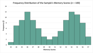
From looking at this graph, we can see that while the average score for the participants is 50.00, very few participants have scores near 50. Instead, the scores form a bimodal distribution with most of the participants’ scores clustering around 46 and 54. By graphing the scores, our interpretation of the data can be enhanced. In this case, the fact that our sample has a bimodal distribution might be an indication that our sample is made up of two different groups, and whatever distinguishes those groups also may interact with either of our variables. For example, our sample may have somehow ended up with roughly a 50-50 mix of college students and older adults, and as a result, the sleep deprivation impacted each group differently (maybe college students are used to being sleep-deprived). Alternatively, our sample may have somehow ended up with roughly 50-50 mix of people with excellent memory skills and people with average memory skills, and as a result, the sleep deprivation may have reduced memory scores for everyone, but the impairment of the people with excellent memory skills was not enough to make them below average.

This step is not typically shared when researchers publish their research findings. It is assumed that the researchers have performed this step, but this assumption may not always be reasonable. For the purposes of this textbook, we will endeavor to include the step where appropriate to reinforce its importance.

4. Compute the Test Statistic

Once we have stated our hypotheses, determined our criteria for making a decision, and collected our data, we are now ready to apply inferential statistics to our data. We do this by calculating a test statistic. There are a number of different test statistics that researchers can use. The specific test statistic needed will depend on the type of data and research methodology. This textbook will cover 7 test statistics, including some of the most commonly used ones.

In this chapter, we will use a test statistic that we actually already know: the z-score. Up to this point, we have primarily used the z-score as a descriptive statistic, but we will now be able to use it as an inferential statistic.

This step of the hypothesis testing system is the main one that involves calculations. The exact formulas that will be used will depend on the appropriate test statistic. Because we are using the z-score, we simply need two formulas:

[latex]\sigma_{_{\!M}} = \frac{\sigma}{\sqrt n}[/latex]

[latex]z = \frac{M - \mu}{\sigma_{_{\!M}}}[/latex]

Often, we will have already calculated the standard error ([latex]\sigma_{_{\!M}}[/latex]) during step 2 when we are drawing the distribution of sample means. Once that has been calculated, we can then calculate the z-score.

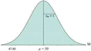
The z-score will ultimately tell us whether or not the sample in the study has an average score (mean) that is substantially different than what the null hypothesis would predict. To show how it does this, let’s continue with our study on sleep deprivation and memory and assume that our group of 100 participants ended up with an average memory score of M = 47.85. At first glance, it appears that our participants ended up with an average memory score that is less than the typical average on the memory test (μ = 50). While this seems to support the idea that sleep deprivation will have an impact on memory, we have to remember that sampling error is a possible explanation for this result. In other words, it is possible that we just happened to sample a group of 100 people who have worse memory skills than average and that’s why they scored so low as a group.

One way to think of it is that we have two possible reasons to explain why our sample had an average memory score of M = 47.85:

1. Sleep deprivation caused them to perform worse on the memory test, or
2. Sleep deprivation had nothing to do with their performance; we just happened to sample a group of people who had poor memory skills on average.

We can’t know for sure which one is correct, but this is where our inferential statistics come in. By calculating the test statistic (in this case, a z-score) we can determine the probability of the second option and thus make an educated decision.

In this chapter, we are using the z-score as our test statistic. Using the mean of M = 47.85, let’s calculate our standard error ([latex]\sigma_{_{\!M}}[/latex]) and our z-score:

[latex]\sigma_{_{\!M}} = \frac{\sigma}{\sqrt n} = \frac{10}{\sqrt 100} = \frac{10}{10} = 1.00[/latex]

[latex]z = \frac{M - \mu}{\sigma_{_{\!M}}} = \frac{47.85 - 50}{1.00} = \frac{-2.25}{1.00} = -2.25[/latex]

Now, let’s apply what we know about z-scores to help us understand what this result describes. A z-score of -2.25 indicates that our sample mean of M = 47.85 is 2.25 standard deviations (in this case, the standard deviation of the sample means – [latex]\sigma_{_{\!M}}[/latex] – or “standard error”) below the mean.

It can help to look at the formula to unpack this interpretation. Starting with the numerator, we subtracted the sample mean (M) and the population mean (μ). In mathematics, subtraction is simply a way of looking for a difference. Thus, we were looking to see if there was a difference between the sample mean (the average memory scores of our sample of 100 people who experienced sleep deprivation, M = 47.85) and the population mean (the average memory score for people who haven’t experienced sleep deprivation, μ = 50). We found that there was a difference of -2.25. This means that our sample mean deviated from the population mean by 2.25 points in the negative direction. Or, in other words, the sample of 100 people who experienced sleep deprivation had an average memory score that was 2.25 points lower than we would have expected if they hadn’t experienced sleep deprivation.

While this difference would likely make us start to wonder if sleep deprivation impacted the memory scores, it is important to remember that sampling error is a possible explanation for this difference. That is where the denominator of the z-score comes in because it includes the standard error ([latex]\sigma_{_{\!M}}[/latex]), which as we discussed in the previous chapter, is technically a measure of the average amount of sampling error we can expect. Thus, in our study with a sample of n = 100 and a population standard deviation of σ = 10, we can expect about 1.00 points of sampling error in the memory scores. This means that if we were to take a random sample of 100 people from a population of memory scores that has a mean of μ = 50 and a standard deviation of σ = 10, we would expect that the sample of 100 people would have an average score of about M = 50 plus or minus about 1.00 points of sampling error. This is how we ended up with the theoretical distribution of sample means based on the central limit theorem of all the possible sample means we could get:

Each of the tiny boxes in the distribution reflects a potential sample mean. Notice that there are a lot of sample means near 50, and there are fewer sample means the farther we get from 50. That should make sense because the average score on this memory test is 50, so we should expect a lot of individuals in our sample of 100 to have scores close to 50. While it is certainly possible that we could get some individuals in our sample who have extremely high memory scores, they will likely be balanced out by some individuals who have extremely low memory scores. Thus, when we average all 100 scores, the group is likely to have a sample mean pretty close to 50. Yet, every once in a while, we could get a random sample of 100 people where we have an unusual number of high memory scores or low memory scores, resulting in the rare sample mean that is extremely low or high, or near the edges of our distribution.

If we now look at our distribution of sample means and include a sample mean of M = 47.85, we get the following:

To more easily see, let’s zoom in on the location of a sample mean of M = 47.85 in this distribution, where we have shaded one of the sample means in orange:

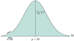
This distribution helps us visualize all of the possible sample means that we could get without any kind of treatment effect. It also helps us to see that while a sample mean of M = 47.85 is certainly possible without any treatment effect, it is a pretty unusual result. For one, it is not very close to 50, which is what we would expect most of the time. Second, it is a pretty rare result. As we get to that end of the distribution, we can see that there are fewer and fewer potential sample means as we move away from the population mean of μ = 50.

So now the question becomes, is this sample mean substantially different from what we expect? And that takes us to the last step.

5. Make a Statistical Decision

In this step, we will combine some of the previous steps. Specifically, we will take the result of Step 4, where we calculated the test statistic for our sample mean, which resulted in a z-score of z = -2.25, and see if that z-score falls in the critical region we determined in Step 2.

Essentially, in order to answer the question, “Is this sample mean substantially different from what we expect?” we will use the “line in the sand” that we drew in Step 2 and see if the test statistic for our sample mean crossed that line. In other words, is our test statistic in the critical region?

Let’s use the directional hypothesis with an alpha of α = 0.05 example from Step 2, where we determined that the “line in the sand” that determined our critical region was the critical value of z_critical = -1.65:

This graph shows us that any sample mean that has a z-score greater than -1.65  does not fall into the extreme 5% of low scores. As a result, a sample mean with a z-score greater than -1.65 would not be considered substantially different from what the null hypothesis would predict. Based on how that sample of participants performed, we would then make the educated guess that their sample mean was probably due to sampling error. In other words, it seems to support the null hypothesis.

On the other hand, any sample mean that has a z-score less than or equal to -1.65  does fall into the extreme 5% of low scores. As a result, a sample mean with a z-score less than or equal to -1.65 would be considered substantially different from what the null hypothesis would predict. Based on how that sample of participants performed, we would then make the educated guess that their sample mean was probably not due to sampling error. In other words, it seems to conflict with the null hypothesis.

What is nice about this step (but also one of the concerns about NHST) is that the researcher’s decision is black-and-white. If the test statistic calculated in Step 4 does not cross the line(s) determined in Step 2, you make one decision, but if it does cross the line(s), you make another decision.

What is difficult about this step is that the wording of the decisions is somewhat confusing due to the use of double-negatives and triple-negatives. The two possible decisions that the research can make are:

• Reject the Null Hypothesis
• Fail to Reject the Null Hypothesis

Reject the Null Hypothesis

We will reject the null hypothesis (or “reject the null”) when the test statistic is in the critical region. In other words, the sample mean was substantially different from what the null hypothesis would predict, and thus, we conclude that the null hypothesis is probably wrong.

Because the null hypothesis usually argues that there is no effect, difference, or correlation, we are, in essence, saying that our data may support the idea of an effect, difference, or correlation.

The phrase “reject the null hypothesis” is a double-negative. It can be understood to be saying: “Say no (reject) to there being no effect, difference, or correlation (null hypothesis).” We call this a double-negative because there are two “no’s” in the sentence. Those two “no’s” can essentially be seen to cancel each other out and we are left with: “Say there is an effect, difference, or correlation.”

However, we can’t actually argue that we’ve proved that there is an effect, difference, or correlation. At best, we could say that our data indicates that we can’t dismiss the idea that there might be an effect, difference, or correlation. Further research on the alternative hypothesis would be warranted.

Fail to Reject the Null Hypothesis

We will fail to reject the null hypothesis, or “retain the null,” when the test statistic is not in the critical region. In other words, the sample mean was not substantially different from what the null hypothesis would predict, and thus, we conclude that the null hypothesis is probably correct.

Because the null hypothesis usually argues that there is no effect, difference, or correlation, we are, in essence, saying that our data may support the idea that there is no effect, difference, or correlation.

The phrase “fail to reject the null hypothesis” is a triple-negative. It can be understood to be saying: “Say no (fail) to saying no (reject) to there being no effect, difference, or correlation (null hypothesis).” We call this a triple-negative because there are three “no’s” in the sentence. Two of those “no’s” can essentially be seen to cancel each other out and we are left with: “Say no to there being an effect, difference, or correlation.”

However, we can’t actually argue that we’ve proved that there is no effect, difference, or correlation. At best, we could say that our data indicates that there might not be an effect, difference, or correlation. Further research on the alternative hypothesis would be questionable unless there were flaws in the research methodology.

Directional or One-Tailed Hypothesis Decisions

If a research is using a directional or one-tailed hypothesis, there will only be one critical region. As discussed in Step 2, the location of that tail (to the left or to the right) will be determined by the alternative hypothesis.

For example, in our example study exploring the impact of sleep deprivation on memory, the alternative hypothesis predicts that sleep deprivation will reduce memory. Thus, the tail would be to the left. Thus, we would end up with the following regions:

As you can see in this picture, if you end up with a sample mean that has a z-score that is greater than -1.65 (did not cross “the line in the sand”), that would tell you that your sample is consistent with the null hypothesis, and you would “fail to reject the null hypothesis” or “retain the null.”

On the other hand, if you end up with a sample mean that has an extremely low z-score that is less than or equal to -1.65 (crossed “the line in the sand”), that would tell you that your sample is inconsistent with the null hypothesis, and you would “reject the null hypothesis” or “reject the null.”

Remember that directional or one-tailed hypotheses specify the direction of an effect, difference, or correlation, so it is also possible to specify a positive effect, difference, or correlation, resulting in a tail to the right:

As you can see in this picture, if you end up with a sample mean that has a z-score that is less than +1.65 (did not cross “the line in the sand”), that would tell you that your sample is consistent with the null hypothesis, and you would “fail to reject the null hypothesis” or “retain the null.”

On the other hand, if you end up with a sample mean that has an extremely high z-score that is more than or equal to +1.65 (crossed “the line in the sand”), that would tell you that your sample is inconsistent with the null hypothesis, and you would “reject the null hypothesis” or “reject the null.”

Non-Directional or Two-Tailed Hypothesis Decisions

If research is using a non-directional or two-tailed hypothesis, there will be two critical regions. Those two tails will be at both extremes (the extreme low scores and the extreme high scores).

For example, in our example study exploring the impact of sleep deprivation on memory, the non-directional or two-tailed alternative hypothesis predicts that sleep deprivation will impact memory. That means that it can either increase memory or it can decrease memory. Thus, the tails will include both of those extremes. Thus, we would end up with the following regions:

As you can see in this picture, if you end up with a sample mean that has a z-score that is greater than -1.96 or less than +1.96 (did not cross either of “the lines in the sand”), that would tell you that your sample is consistent with the null hypothesis, and you would “fail to reject the null hypothesis” or “retain the null.”

On the other hand, if you end up with a sample mean that has an extreme z-score that is less than or equal to -1.65 (crossed “the line in the sand”) or more than or equal to +1.65 (crossed “the line in the sand”), that would tell you that your sample is inconsistent with the null hypothesis, and you would “reject the null hypothesis” or “reject the null.”

6. Share the Results

The final step of hypothesis testing is to share the results with the research community. The Scientific Method is ultimately a social endeavor because it is strengthened by researchers sharing and debating the results. It is through this social process that science helps us get closer to the truth.

For our purposes, we will focus on how the statistical results are typically reported in the research literature, usually in the Results section of original empirical research articles published in peer-reviewed research journals. Through learning how statistical results are written, we are able to learn how to better read and interpret the results.

Reporting our results in the research literature will differ for each of the different test statistics. In this textbook, each chapter that covers a test statistic will provide an example report, as well as some tips about how to write them for different research questions and hypotheses. Thankfully, though, there are some commonalities between the different test statistics.

In this chapter, we used the z-score as the test statistic. Let’s use our example result where our sample of n = 100 individuals ended up with a sample mean of M = 87.85 on the memory test after experiencing sleep deprivation. In Step 4, we determined that the z-score for that sample mean was z_observed = -2.25, and in Step 5, we determined that this z-score is in the critical region. As a result, we would “reject the null hypothesis” and conclude that “sleep deprivation probably impaired memory.” This would then get translated to the following report in the literature: