
4.2 – Deviations and the Concept of an Average Deviation
In order to get a more precise measure of spread we need to calculate what is called the standard deviation. The standard deviation measures the average amount that all the individuals in the distribution deviate from the mean. This definition may not make a lot of sense, so let’s break it down to a key component: a deviation.
A deviation is the amount of difference between an individual score and the mean for the group. To calculate it, just subtract an individual’s score from the mean:
[latex]\text{Deviation}=X-\mu[/latex]
Let’s work with one of our previous distributions of scores:
2, 3, 3, 3, 4, 6, 7, 7, 7, 8
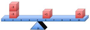
Suppose we want to know how much the score of X = 6 deviates from the mean. First, we need to calculate the mean for the distribution:
[latex]\mu=\frac{\Sigma X}{N}=\frac{2+3+3+3+4+6+7+7+7+8}{10}=\frac{50}{10}=5[/latex]
The average score for this group was μ = 5.
Now, suppose we want to calculate how much one of the scores in that group deviates from the mean of 5. Let’s use the score of X = 6. All we need to do is take that score and subtract the mean:
[latex]\text{Deviation}=X-\mu=6-5=+1[/latex]
This tells us that the score of X = 6 has a deviation of +1.
If we then calculate the deviation for the score of X = 2 …
[latex]\text{Deviation}=X-\mu=2-5=-3[/latex]
This tells us that the score of X = 2 has a deviation of -3.
You will see that positive deviations tell you that a score is above the mean, while negative deviations tell you that a score is below the mean. Thus, the score of X=6 is one point above the mean of 5, while the score of X = 2 is three points below the mean of 5.
Hopefully, you can start to see that these deviations give us a sense of spread. Higher deviations, regardless of the sign (+/−), are farther from the mean and thus more spread out, while smaller deviations are closer to the mean and thus less spread out. From the example above, the score of X = 2 is farther from the mean (3 points away) than the score of X = 6 (only 1 point away).
However, these deviation scores just give us an indication of the distance from the mean for each individual score. What if we want to know the spread for a group of scores, (which is the whole point of having a measure of spread)?
Given that the number that we get from a deviation calculation is a measure of distance or spread from the mean, what if we took the average of all the deviations in a distribution? If most of the scores are close to the mean, meaning they are not spread out and thus have a lot of small deviations, then you should have a small average deviation. If most of the scores are far from the mean, meaning they are very spread out and thus there are a number of large deviations, then you should have a large average deviation.
It turns out that this is the meaning of standard deviation. The word “standard” is simply being used like the word “average.” We are simply going to calculate the average deviation from the mean for a group of scores.
It turns out, however, that the calculation of an average deviation, or standard deviation, is not as simple as it sounds. Typically, in order to calculate a mean we just add up all the scores and divide by the number of scores. For the deviations, this would mean adding up all the deviations and then dividing by the number of deviations.
Unfortunately, it’s in the adding up of all the deviations where we run into trouble. To show you the problem, let’s calculate all the deviations for a sample of N = 10 scores that has a mean of μ = 5. Below we have all of the scores laid out in one column of a table, with the deviation next to it:
| X | Deviation (X-μ) |
| 8 | 8 – 5 = +3 |
| 7 | 7 – 5 = +2 |
| 7 | 7 – 5 = +2 |
| 6 | 6 – 5 = +1 |
| 5 | 5 – 5 = 0 |
| 4 | 4 – 5 = -1 |
| 4 | 3 – 5 = -1 |
| 4 | 3 – 5 = -1 |
| 3 | 3 – 5 = -2 |
| 2 | 2 – 5 = -3 |
Now, if we add up all of the deviations, it equals zero:
3 + 2 + 2 + 1 + 0 + (-1) + (-1) + (-1) + (-2) + (-3) = 0
This is not a coincidence. It will happen every time we add up the deviations. Remember that the mean is the balance point for the scores in the distribution so that the amount of deviation above the mean and below the mean are equal.
The deviations will always add up to zero. This is a problem if we want to calculate the average deviation. Essentially all the negative deviations cancel out all the positive deviations.
Statisticians, however, have figured out a mathematical workaround for this problem. In order to get handle the negative numbers canceling everything out, they decided to square all the deviations. If you square a number, you simply multiply the number by itself. Thus, because a negative number times a negative number equals a positive number, all our negative deviations are eliminated. So if we have a deviation of -3, and we square it, we will end up with a positive number:
[latex]\text {Squared Deviation} =(X-\mu)^2=(-3)^2=+9[/latex]
We can then do that for all of our scores:
| X | Deviation (X-μ) | Squared Deviation (X-μ)2 |
| 8 | 8 – 5 = +3 | (8 – 5)2 = (+3)2 = 9 |
| 7 | 7 – 5 = +2 | (7 – 5)2 = (+2)2 = 4 |
| 7 | 7 – 5 = +2 | (7 – 5)2 = (+2)2 = 4 |
| 6 | 6 – 5 = +1 | (6 – 5)2 = (+1)2 = 1 |
| 5 | 5 – 5 = 0 | (5 – 5)2 = (0)2 = 0 |
| 4 | 4 – 5 = -1 | (4 – 5)2 = (-1)2 = 1 |
| 4 | 3 – 5 = -1 | (3 – 5)2 = (-1)2 = 1 |
| 4 | 3 – 5 = -1 | (3 – 5)2 = (-2)2 = 4 |
| 3 | 3 – 5 = -2 | (3 – 5)2 = (-2)2 = 4 |
| 2 | 2 – 5 = -3 | (2 – 5)2 = (-3)2 = 9 |
You can see that all of the squared deviations are positive. This then allows us to add up all the squared deviations (which is what we would want to do in order to calculate an average):
9 + 4 + 4 + 1 + 0 + 1 + 1 + 4 + 4 + 9 = 37
We have technically just calculated a thing that we will call Sum of Squares (SS). Sum of Squares is short for “the sum of the squared deviations.” Then, if we divide this Sum of Squares by the total number of scores, we will then have calculated the average squared deviation, which is what statisticians call variance.
[latex]\text{Variance} =\sigma^2= \frac{X-\mu}{N}=\frac{37}{10} = 3.70[/latex]
However, our goal wasn’t to know the average squared deviation. We wanted to know the average deviation (without the square). Well, because we squared the deviations in order to avoid having them cancel each other out, we will simply take the square root of the variance to get the average deviation, or what is called the “standard deviation.”
[latex]\text{Standard Deviation} =\sigma = \sqrt{\sigma^2}=\sqrt{3.70}=1.924[/latex]
Thus, the scores in our distribution had an average deviation from the mean of about 1.924 points. If you look at all the deviations in the middle column of the table above (again ignoring the sign +/-), you can see that 1.924 is a pretty good description of the average deviation with the deviations ranging from 0 to 3. Ultimately, this standard deviation gives us an excellent measure of the spread of this distribution of individuals’ scores. Their scores deviate from the mean by an average of 1.924 points.
Now imagine we had a slightly different set of scores:
| X | Deviation (X-μ) | Squared Deviation (X-μ)2 |
| 80 | 80 – 50 = +30 | (80 – 50)2 = (+30)2 = 900 |
| 70 | 70 – 50 = +20 | (70 – 50)2 = (+20)2 = 400 |
| 70 | 70 – 50 = +20 | (70 – 50)2 = (+20)2 = 400 |
| 60 | 60 – 50 = +10 | (60 – 50)2 = (+10)2 = 100 |
| 50 | 50 – 50 = 0 | (50 – 50)2 = (0)2 = 0 |
| 40 | 40 – 50 = -10 | (40 – 50)2 = (-10)2 = 100 |
| 40 | 30 – 50 = -10 | (30 – 50)2 = (-10)2 = 100 |
| 40 | 30 – 50 = -10 | (30 – 50)2 = (-20)2 = 400 |
| 30 | 30 – 50 = -20 | (30 – 50)2 = (-20)2 = 400 |
| 20 | 20 – 50 = -30 | (20 – 50)2 = (-30)2 = 900 |
If we add up the squared deviations, which is Sum of Squares (SS), we will get:
900 + 400 + 400 + 100 + 0 + 100 + 100 + 400 + 400 + 900 = 3700
Then if we calculate the average of those squared deviations, which is Variance (σ2), we will get:
[latex]\text{Variance} =\sigma^2= \frac{X-\mu}{N}=\frac{3700}{10} = 370[/latex]
Then if we take the square root of the average squared deviation to get the average squared deviation, which is standard deviation (σ), we will get:
[latex]\text{Standard Deviation} =\sigma = \sqrt{\sigma^2}=\sqrt{370}=19.235[/latex]
If you look at all the deviations in the second column of the table above, you can see that they range from 0 to 30 points, or 0 to 30 points away from the mean. In other words, these scores are more spread out. This is reflected in the standard deviation with is now larger than our previous example. We now know that the average deviation, or the standard deviation, is 19.235 points.
Steps to Calculate Standard Deviation
As we saw above, the standard deviation is an excellent measure of the spread of a group of scores. A group of individuals with a small standard deviation has scores that are very close to each other and not very spread out, while a group of individuals with a large standard deviation has scores that are generally far from each other and are very spread out. Now that we have introduced the concept of standard deviations in order to understand what it captures, let’s take a step back and try to formalize our process for the calculation.
First, remember that the process of calculating a standard deviation is not very direct because, as we saw in the previous section, our deviations added to zero and we had to use a workaround. Thus, we will follow three steps:
- Calculate the Sum of Squares
- Calculate the Variance
- Calculate the Standard Deviation
The average amount of deviation from the mean for a group of scores. The higher the standard deviation, the more a group of scores deviates from the mean for the group, and thus the more the scores vary (or are spread out).This is one of the most useful measures of variability.
A measure of the distance between an individual's score and the mean for the group. In other words, how much does the individual's score "deviate" from the group average.
The sum a group of squared deviations. It is a step that we use to calculate variance and standard deviation, but it also is a measure of variability or spread.
The average squared deviation. This is a common measure of variability or spread. The higher the number, the more variability. However, it is difficult to interpret as a descriptive statistic.

Feedback/Errata