6.8 – Application / Level Up

With the skills we have just learned, we are now able to handle some important and interesting real-world question types:

• How likely is a client or patient to have a score on a given test or measurement (e.g., reading math, body temperature, blood pressure, depression) that is above/below a particular score?
• What score on a given test or measurement would be needed to be in the top/bottom       %?
• How typical/unusual is a client’s or patient’s score on a given test or measurement?

To do this, we needed to know 3 things about the test or measurement we are using:

1. The scores are normally distributed (this allows us to use the Unit Normal Table)
2. The mean score for the group to which the individual is compared
3. The standard deviation for the group to which the individual is compared

If we know these 3 things, we can then use z-score formulas to answer the types of questions above.

For example, let’s say we wanted to research the impact of a newly developed “math pill.” This pill contains certain chemicals that allegedly improve the functioning of both the parietal lobe (involved in understanding numbers) and the prefrontal cortex (involved in working memory and task strategy), and thus the researchers believe that it will improve performance on math problems.

A researcher could randomly sample an individual, give them the “math pill,” and then give them a standardized math achievement test (which measures how well an individual can solve math problems). In psychology, we know that these standardized achievement tests have the following characteristics:

• Scores are normally distributed
• Have a mean of μ = 100
• Have a standard deviation of σ = 15

If the “math pill” actually works, the individual study participant should end up performing better on the standardized math test. Unfortunately, the researcher was not able to determine how well the participant would score on the math test without the “math pill” because they were worried that giving the person the math test both before and after taking the pill would end up helping them do better on the second testing (after the pill). As a result, they only gave the standardized math test after the participant took the “math pill.”

Let’s say the participant in the research study ends up scoring X = 133 on the math achievement test. 

At this point, the researcher will want to examine whether that score is due to the “math pill” or not. A score of X = 133 seems like a pretty high score, given that it is above the mean of μ = 100. And a high score on the math test would seem to support the idea that the “math pill” improves math performance. This would be referred to as a “treatment effect“.

However, we cannot jump to this conclusion because there is another possible explanation for the result. It is simply possible that the participant in the study would have scored the same without the “math pill.” In other words, that score of X = 133 occurred by chance (the researcher happened to randomly sample a participant who has learned a lot of math skills and scores well above average on math achievement tests).

So, at this point, there are two possible explanations for why our participant scored X = 133 on the math test:

• The “math pill” improved their math abilities (a treatment effect).
• The researcher happened to randomly sample a high-scoring individual (chance).

Because there are two possible explanations, the researcher shouldn’t just choose whichever one they prefer. Instead, they can use some of the skills we learned about individual z-scores and probability to garner more information that can be used to help them make a more informed choice between the two options. Specifically, they can find the probability that the result was due to chance, and if that has a very low probability of being the explanation, then the treatment effect (the “math pill” improved math performance) becomes the better choice.

This is where we technically start to get into inferential statistics. Inferential statistics are statistical processes that help researchers explore a research question by calculating statistics and probabilities to infer generalizations about the population from the data and results of a sample.

The process of making statistical inferences is where learning statistics becomes more elusive for most people. Inferential statistics will use:

• statistics, which involve mathematical calculations;
• probability, which is not intuitive for most people; and
• inference, which is a process of drawing a conclusion from known facts.

Through these components, researchers can make conclusions about their research questions, but the process can feel somewhat cloudy and detached from the research question, especially for people new to statistics. However, the better someone understands this process, the better they are at understanding the real meaning behind research results. And (spoiler alert!), the conclusions of research projects are actually just “educated guesses.” They don’t “prove” anything, but rather they either provide “support” or not for a particular hypothesis or theory.

To do this, the researcher would simply apply the skills we learned previous.  First, they can convert that score of X = 133 into a z-score:

[latex]z = \frac{X - \mu}{\sigma} = \frac{133 - 100}{15} = \frac{+33}{15} = +2.20[/latex]

This tells the researcher that the individual’s score is 2.20 standard deviations above the mean, which is a very high score and seems to support the idea that the “math pill” improved the participant’s performance on the math test. However, as we have already noted, this high score could instead be due to chance. And that’s where we can use the Unit Normal Table to determine how whether or not this score on the math test is likely or unlikely to happen by chance. In other words, if we were to randomly select an individual and give them a standardized math achievement test, what is the probability they would score above X = 133?

Because the researcher knows that a score of X = 133 is equal to a z-score of z = 2.20, they can now simply ask the question, what is the probability of an individual having a z-score greater than 2.20?

The researcher can find the answer to this question in the Unit Normal Table, but in order to use it properly, they need to know whether they are looking for a body, a tail, or a slice. This means that they should draw a normal distribution, locate the z-score of z = 2.20, and shade all of the distribution that lies above the z = 2.20:

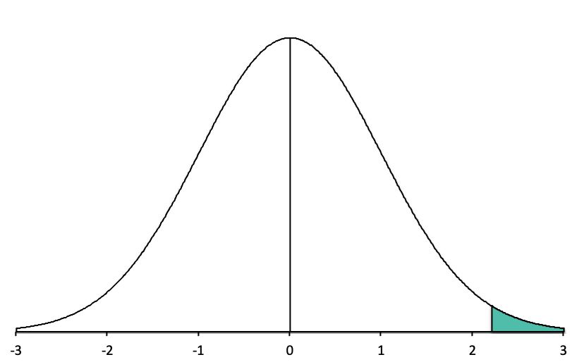From looking at this picture, we can see that the shaded part of the distribution is a tail. So now we look up z = +2.20 in the z-score column of the Unit Normal Table and go across to the Tail column, and we see that the proportion of the shape that is shaded is 0.0139, or about 1.39% of the normal distribution is shaded above a z-score of +2.20.

More importantly, though, this tells the researcher that the likelihood of randomly sampling a person who will score X = 133 (which corresponds to z =+2.20) or higher is 0.0139, or has a 1.39% chance of happening. It means that if someone were to sample 1000 people, only about 14 of them would score this high or higher. That’s a very unlikely thing to happen.

So let’s return to the two possible explanations for the results of the “math pill” research study:

1. The “math pill” improved their math abilities (a treatment effect).
2. The researcher happened to randomly sample a high-scoring individual (chance).

However, we now know that the second option (chance) is only going to happen about 1.39% of the time, and because it is very unlikely, the researcher would be wise to argue for the other option (a treatment effect). In other words, they should argue that the results of the research study support the idea that the “math pill” actually improves math performance.

Now, hopefully, some of you are finding yourself a little skeptical about the researcher’s claim. For some, it’s because they find it highly questionable that there could actually be a pill that someone could take that improves math performance. For others, and this is the skepticism that I hope to instill in you, it’s because the data does not actually prove that the “math pill” works. The researcher is basically making guesses about the results based on the probability of only one of the options that explain the result. And on top of that, it is still actually possible that the researcher happened to sample an individual who was going to score that high without the “math pill,” even if it is a low likelihood (only a 1.39% chance). It’s not impossible.

These issues regarding how research studies use statistics are incredibly important to try to understand (it is worth noting that they are very difficult for many people to understand, especially this early in our coverage of statistics). Here are some useful concepts to remember when trying to understand statistical inferences:

• They are “educated guesses.”
• The conclusions are based on probability and could be wrong.
• They don’t “prove” but rather “provide support” for hypotheses and theories.

I often find it helpful to think of research decisions that utilize statistical inference as “making bets.” Let’s say I offer you the following bet:

Would you take the bet?

You should. We can calculate the probability that the card will be the Queen of Hearts by using our probability formula:

[latex]P (\text{Queen of Hearts}) = \frac{\text{Number of Queen of Hearts in the Deck}}{\text{Total Number of Cards in the Deck}} = \frac{1}{52} = 0.019[/latex]

There is a 1.9% chance that the selected card will be the Queen of Hearts. In other words, you have only a 1.9% chance of losing your $1 bet, and a 98.1% chance of winning $10. Thus, the odds are definitely in your favor, so it would be a good bet to take because you are unlikely to lose.

However, it is important to note that the small (1.9%) probability of losing does not mean that you won’t lose and instead will win. It just means that you are very unlikely to lose and very likely to win.

Research conclusions are the same. If the probability that a research result was due to chance was a very low probability, it does not mean that the research result was not due to chance and instead is due to a treatment effect. It just means that it is very unlikely that it was due to chance and very likely that it was due to the treatment effect.