8.8 – Step 4: Compute the Test Statistic

4. Compute the Test Statistic

Once we have stated our hypotheses, determined our criteria for making a decision, and collected our data, we are now ready to apply inferential statistics to our data. We do this by calculating a test statistic. There are a number of different test statistics that researchers can use. The specific test statistic needed will depend on the type of data and research methodology. This textbook will cover 7 test statistics, including some of the most commonly used ones.

In this chapter, we will use a test statistic that we actually already know: the z-score. Up to this point, we have primarily used the z-score as a descriptive statistic, but we will now be able to use it as an inferential statistic.

This step of the hypothesis testing system is the main one that involves calculations. The exact formulas that will be used will depend on the appropriate test statistic. Because we are using the z-score, we simply need two formulas:

[latex]\sigma_{_{\!M}} = \frac{\sigma}{\sqrt n}[/latex]

[latex]z = \frac{M - \mu}{\sigma_{_{\!M}}}[/latex]

Often, we will have already calculated the standard error ([latex]\sigma_{_{\!M}}[/latex]) during step 2 when we are drawing the distribution of sample means. Once that has been calculated, we can then calculate the z-score.

The z-score will ultimately tell us whether or not the sample in the study has an average score (mean) that is substantially different than what the null hypothesis would predict. To show how it does this, let’s continue with our study on sleep deprivation and memory and assume that our group of 100 participants ended up with an average memory score of M = 47.85. At first glance, it appears that our participants ended up with an average memory score that is less than the typical average on the memory test (μ = 50). While this seems to be in line with the hypothesis that sleep deprivation will have an impact on memory, we have to remember that sampling error is a possible explanation for this result. In other words, it is possible that we just happened to sample a group of 100 people who have worse memory skills than average, and that’s why they scored so low as a group.

One way to think of it is that we have two possible reasons to explain why our sample had an average memory score of M = 47.85:

1. Sleep deprivation caused them to perform worse on the memory test, or
2. Sleep deprivation had nothing to do with their performance; we just happened to sample a group of people who had poor memory skills on average.

We can’t know for sure which one is correct, but this is where our inferential statistics come in. By calculating the test statistic (in this case, a z-score), we can determine the probability of the second option and thus make an educated decision.

In this chapter, we are using the z-score as our test statistic. Using the mean of M = 47.85, let’s calculate our standard error ([latex]\sigma_{_{\!M}}[/latex]) and our z-score:

[latex]\sigma_{_{\!M}} = \frac{\sigma}{\sqrt n} = \frac{10}{\sqrt 100} = \frac{10}{10} = 1.00[/latex]

[latex]z = \frac{M - \mu}{\sigma_{_{\!M}}} = \frac{47.85 - 50}{1.00} = \frac{-2.25}{1.00} = -2.25[/latex]

Now, let’s apply what we know about z-scores to help us understand what this result describes. A z-score of -2.25 indicates that our sample mean of M = 47.85 is 2.25 standard deviations (in this case, the standard deviation of the sample means – [latex]\sigma_{_{\!M}}[/latex] – or “standard error”) below the mean.

It can help to look at the formula to unpack this interpretation. Starting with the numerator, we subtracted the sample mean (M) and the population mean (μ). In mathematics, subtraction is simply a way of looking for a difference. Thus, we were looking to see if there was a difference between the sample mean (the average memory scores of our sample of 100 people who experienced sleep deprivation, M = 47.85) and the population mean (the average memory score for people who haven’t experienced sleep deprivation, μ = 50). We found that there was a difference of -2.25. This means that our sample mean deviated from the population mean by 2.25 points in the negative direction. Or, in other words, the sample of 100 people who experienced sleep deprivation had an average memory score that was 2.25 points lower than we would have expected if they hadn’t experienced sleep deprivation.

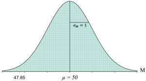
While this difference would likely make us start to wonder if sleep deprivation impacted the memory scores, it is important to remember that sampling error is a possible explanation for this difference. That is where the denominator of the z-score comes in because it includes the standard error ([latex]\sigma_{_{\!M}}[/latex]), which as we discussed in the previous chapter, is technically a measure of the average amount of sampling error we can expect. Thus, in our study with a sample of n = 100 and a population standard deviation of σ = 10, we can expect about 1.00 points of sampling error in the memory scores. This means that if we were to take a random sample of 100 people from a population of memory scores that has a mean of μ = 50 and a standard deviation of σ = 10, we would expect that the sample of 100 people would have an average score of about M = 50 plus or minus about 1.00 points of sampling error. This is how we ended up with the theoretical distribution of sample means based on the central limit theorem of all the possible sample means we could get:

Each of the tiny boxes in the distribution reflects a potential sample mean. Notice that there are a lot of sample means near 50, and there are fewer sample means the farther we get from 50. That should make sense because the average score on this memory test is 50, so we should expect a lot of individuals in our sample of 100 to have scores close to 50. While it is certainly possible that we could get some individuals in our sample who have extremely high memory scores, they will likely be balanced out by some individuals who have extremely low memory scores. Thus, when we average all 100 scores, the group is likely to have a sample mean pretty close to 50. Yet, every once in a while, we could get a random sample of 100 people where we have an unusual number of high memory scores or low memory scores, resulting in the rare sample mean that is extremely low or high, or near the edges of our distribution.

If we now look at our distribution of sample means and include a sample mean of M = 47.85, we get the following:

To more easily see, let’s zoom in on the location of a sample mean of M = 47.85 in this distribution, where we have shaded one of the sample means in orange:

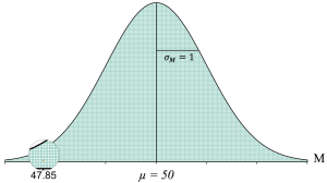
This distribution helps us visualize all of the possible sample means that we could get without any kind of treatment effect. It also helps us to see that while a sample mean of M = 47.85 is certainly possible without any treatment effect, it is a pretty unusual result. For one, it is not very close to 50, which is what we would expect most of the time. Second, it is a pretty rare result. As we get farther from the middle of the distribution, we can see that there are fewer and fewer potential sample means as we move away from the population mean of μ = 50.

So now the question becomes, is this sample mean substantially different from what we expect? And that takes us to the last step.