
7.2 – Distribution of Sample Means
Back in the chapter on frequency distributions, we learned how to create frequency tables and frequency graphs to organize and describe our data.
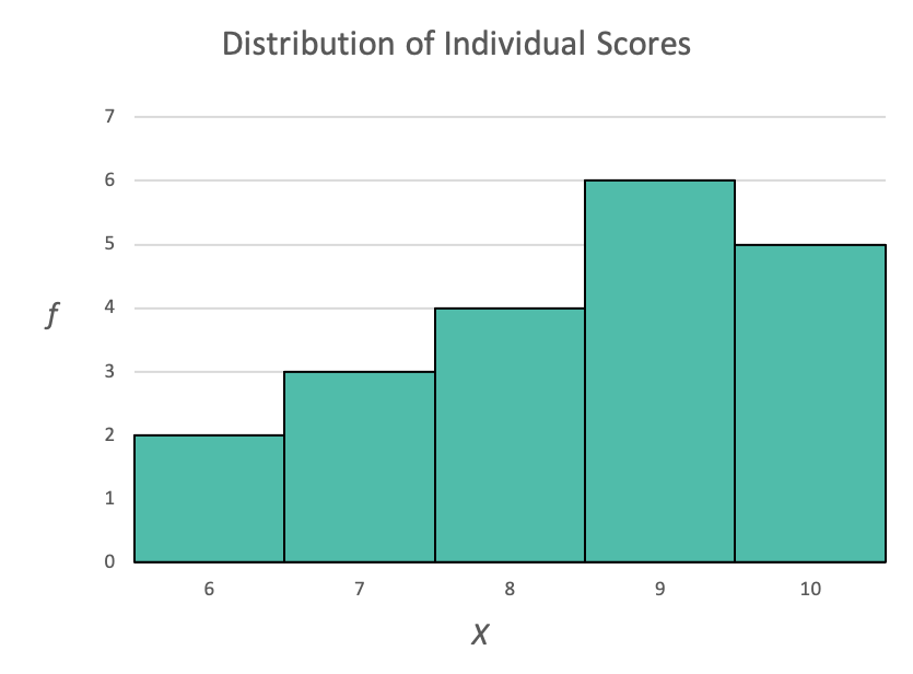
Technically, graphs like the histogram above could be called distributions of individual scores (or X's). In other words, they were graphs or tables that organized and described how a group of people scored as individuals. For example, in the above histogram, we know that there were:
- 2 individuals who scored 6,
- 3 individuals who scored 7,
- 4 individuals who scored 8,
- 6 individuals who scored 9, and
- 5 individuals who scored 10.
It is also possible for statisticians to create frequency distributions that depict other statistics, not just individual scores (X). For example, if you were to sample a group of people from a population and then calculate a statistic (e.g., mean, standard deviation, median, etc.) for that sample, you could technically start to create a graph of that statistic if you were to repeatedly take more samples from that same population and calculate the statistic for each of those samples. The resulting distribution graph or table is called a sampling distribution.
Let's explore an example to help this make more sense.
Suppose that we want to find out the average age of students in our statistics class. Because our class is relatively small, we can easily ask each student to report their age and then calculate the mean for that data. Imagine that in our class (N = 20), students reported the following ages:
| Age (X) |
| 20 |
| 22 |
| 18 |
| 19 |
| 35 |
| 17 |
| 19 |
| 26 |
| 34 |
| 20 |
| 22 |
| 18 |
| 19 |
| 20 |
| 42 |
| 19 |
| 20 |
| 61 |
| 21 |
| 18 |
We can then calculate the mean age by adding up every student's age (ΣX) and then dividing by the total number of students (N):
[latex]\mu = \frac{\Sigma X}{N} = \frac {490}{20} = 24.50[/latex]
We now know that the mean age of students in our statistics class is 24.50 years of age. Because our research question was about the age of students in our statistics class, the population would technically be the 20 students in our statistics class. And because we calculated the mean using all of the students in our statistics class, we have technically calculated the population mean (μ). And as discussed back in the first chapter, we have conducted a census, and our mean is not a statistic but is rather a parameter.
In order to explore the idea of sampling distributions, we are now going to take a sample of n = 4 people from the population of our class. Suppose that I happen to randomly select the first 4 students from the above list, with the following ages:
| Age (x) |
| 20 |
| 22 |
| 18 |
| 19 |
We can now calculate the mean for this sample of students by adding up all of their ages (Σx) and dividing it by the number of students in this sample (n):
[latex]M = \frac{\Sigma x}{n} = \frac {79}{4} = 19.75[/latex]
We now know that the mean age of the students in our sample is 19.75 years of age. And because we calculated this based upon a sample it is technically known as a sample mean, and it is a statistic.
Suppose now that we then repeat this process 9 more times, sampling 4 students from our class and calculating the sample mean each time. We might end up with the following results:
| X1 | X2 | X3 | X4 | Sample Mean (M) |
| 20 | 22 | 18 | 19 | M1 = 19.75 |
| 19 | 34 | 42 | 18 | M2 = 28.25 |
| 22 | 17 | 26 | 19 | M3 = 21.00 |
| 18 | 19 | 19 | 34 | M4 = 22.50 |
| 22 | 22 | 34 | 20 | M5 = 24.50 |
| 42 | 18 | 19 | 20 | M6 = 24.75 |
| 17 | 20 | 34 | 26 | M7 = 24.25 |
| 26 | 42 | 19 | 18 | M8 = 26.25 |
| 20 | 19 | 34 | 22 | M9 = 23.75 |
| 61 | 19 | 18 | 19 | M10 = 29.25 |
From these results, we can see that these sample means vary quite a bit, both from each other and also from the population mean. Whenever a sample statistic (in this case, a sample mean) is different from the population parameter (in this case, the population mean) that is considered to be due to sampling error. For example, our first sample had a sample statistic of M = 19.75 years of age, which is younger than the population parameter of μ = 24.50 years of age. We can explain this difference as being due to the fact that we happened to randomly sample 4 students who happened to be younger on average. For the second sample, its sample mean is M = 28.25years of age, which is older than the population parameter of μ = 24.50 years of age. Again, this is due to sampling error and the second sample happened to be older on average.
While the phrase "sampling error" sounds like a mistake, it is better to think of it as an expected pattern when sampling from a population. Most samples tend to have some sampling error because they are simply not perfectly representative of the population. Fortunately, this pattern can be used to our advantage if we can understand the pattern.
To understand the pattern of samples and sampling error, statisticians used sampling distributions to create a graph of a sample statistic to visualize the results of sampling.
If we look at the far-right column in the above table, we see 10 sample means. Let's create a histogram using groups (e.g., sample means between 23 and 24, etc.) of those 10 numbers:
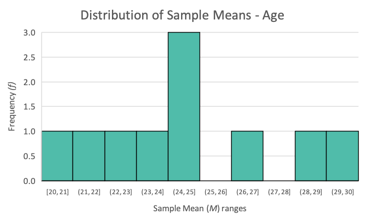
We now have a visual depiction of where the 10 sample means tended to fall. What we've created is technically called a distribution of sample means.
Are there any patterns you see when looking at these 10 sample means? One thing that should stand out is that there is a big group of sample means in the middle of all of the sample means. In fact, those 3 sample means fall in the 24-25 range. All of the other ranges have no more than 1 sample mean. Given that the population mean of μ = 24.50 is right in the middle of that 24-25 range, it appears there are more sample means near the population mean.
Even though we have taken a very small set of samples (only 10) from our class population, we can still start to identify some interesting patterns. Thankfully, so that we don't have to do it ourselves, statisticians have performed similar sampling demonstrations with huge numbers of samples of a given size and the results demonstrate the following patterns in sample means:
- Sample means tend to bunch up around the population mean.
- As you get farther from the population mean in either direction, you get few sample means.
- Larger sample sizes result in less distance between the sample means and the population mean on average.
Much of this should make sense. First, sample means would likely be closer to the population mean in general because they come from the population, and thus they should reflect the population even with sampling error (for example, a sample mean from our class should still reflect the population and should not be something like 1,264 - it should be around 24.50).
Second, while we can end up with a sample mean that is very far from our population mean of μ = 24.50, it just isn't very likely. If we sampled the four oldest people from our class (ages 61, 42, 35, and 34), they would have an average age of M = 43.00. Clearly, that sample mean is very different from the population mean of μ = 24.50. However, it can only happen if we sampled those exact four students, so it is very unlikely to happen much, like with any sample means that are farther from the population mean.
Finally, we have learned before that larger samples tend to be more representative of the population (while it's not always true because biased samples won't be representative regardless of the size, it is a good general rule to use), and thus a larger sample should then have less sampling error. If we reduce sampling error, we reduce how far away the sample means are from the population mean, which then reduces the spread of the sample means.
Now that we have tried to get a sense of sampling and the predictable patterns in the distributions of sample means, we are going to learn about a statistical theorem that essentially formalizes these patterns we've noticed, called the central limit theorem.
A frequency distribution of a statistic (e.g., mean, standard deviation, etc.) calculated for a set of samples.
The group of individuals or objects that are the focus of a research question.
Example: For the research question: "Does caffeine increase attention of people with Attention Deficit Disorder?" the population is "people with Attention Deficit Disorder."
The average score for all of the individuals in the population of interest (which is based upon the research question).
A research study that measures every individual in the population of interest.
A measurement based upon a sample taken from the population of interest.
A measurement based upon all of the individuals in the population of interest.
The average score of the individuals in a sample.
An explanation for the difference between a sample statistic and the corresponding population parameter.
A sampling distribution that depicts a number of sample means of a given size (n) taken from the same population.

Feedback/Errata