6.7 – Finding Individual Scores (X) from Percentages

In this section, we are going to start with skills we learned in the previous section:

• draw a normal distribution
• locate and shade a percentage of the distribution
• identify the type of shaded area (e.g., body, tail, slice)
• convert the percentage to a proportion
• lookup the proportion/probability in the Unit Normal Table
• identify the z-score cutoff(s)

And then, we are going to add:

• use z-score formulas from the previous chapter.

This combination will allow us to answer more typical questions from the real world of research and practice. To do this, we just need to add a couple more steps to what we used in the previous section:

From a Percentage to a Single Individual Score (X)

Suppose you are in charge of hiring at your law firm. Your firm is a very prestigious law firm and only wants to hire the best new lawyers fresh out of law school. However, your firm receives thousands of applications each year and doesn’t have time to review and interview all candidates, so you decide to use applicants’ scores on the Multistate Bar Examination (MBE) and screen for individuals with scores in the top 10% on the bar exam. Thus, you will want to answer the following question:

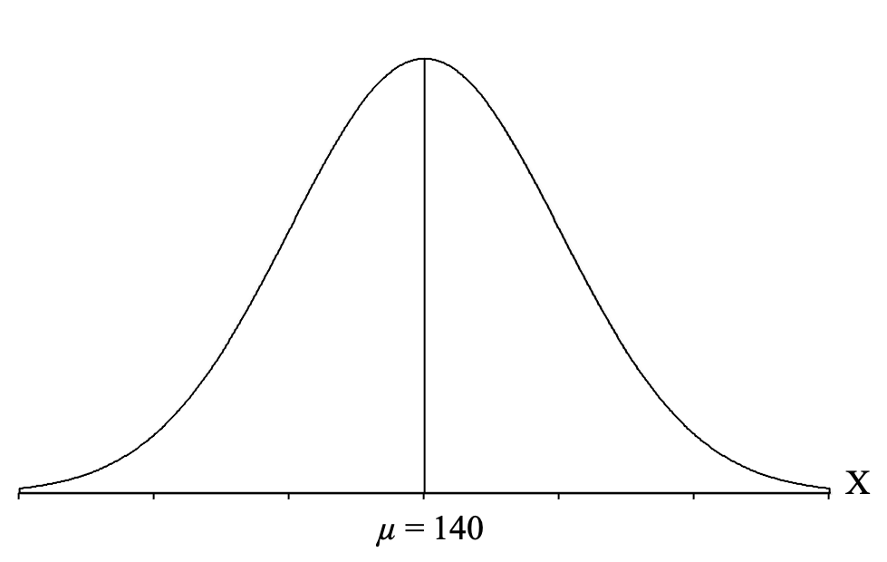
We start by drawing the normal distribution and labeling it with an “X” on the right, to indicate that it is a distribution of individual scores.

Then we draw a vertical line in the middle to represent the mean. We can label this vertical line with the population mean (μ) given in the question, which for the MBE is μ = 140.

Then we identify the part of the distribution specified in the question, which for our question is the “top 10%.” “Top” means on the right-hand side of the distribution because that is where the higher, or “top,” scores are located (remember that the x-axis is a number line and higher scores are to the right). So we want to shade 10% of our distribution starting from the right-hand side:

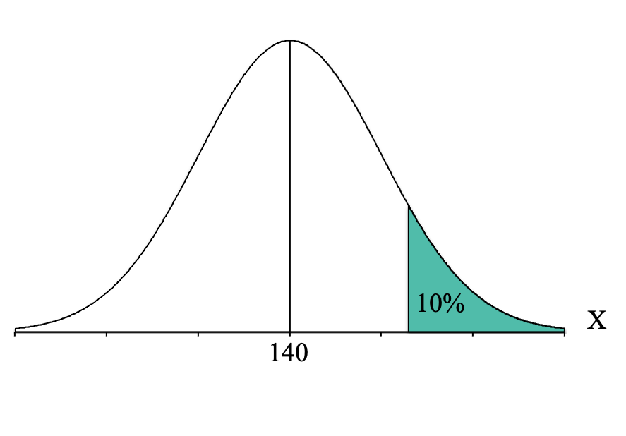
Looking at that picture, we can see that the shaded area is a “tail.” We then need to convert our percentage to a proportion. To convert our percentage of 10% to a proportion we simply divide it by 100. Thus, we look for the proportion of 0.1000 (make sure to use four decimal places because the proportions in our Unit Normal Table go to four decimal places).

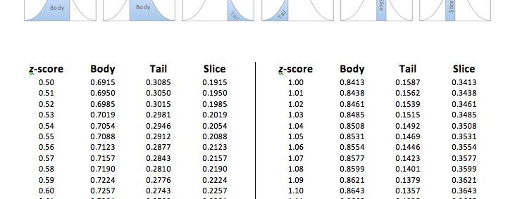
As you can see in the table, the exact proportion of 0.1000 does not exist in the Tail column. The two closest proportions to 0.1000 are 0.1003 and 0.0985. At this point, we then pick the proportion that is the closest to our proportion. By subtracting each of the proportions in the table from our proportion of 0.1000 we find that the proportion of 0.1003 is 0.0003 or three ten-thousandths away, while the proportion of 0.0985 is 0.0015 or fifteen ten-thousandths away:

[latex]\begin{tabular}[c]{r} 0.1003\\ - 0.1000\\ \hline 0.0003 \end{tabular}[/latex]          [latex]\begin{tabular}{r} 0.1000\\ - 0.0985\\ \hline 0.0015 \end{tabular}[/latex]

Thus, the proportion of 0.1003 is a little bit closer. So now we use the proportion of 0.1003 and simply go across that row to the z-score column to find the z-score cutoff. We have now determined that the z-score cutoff for the top 10% is at z = 1.28.

However, it is important to recognize that we are NOT looking for the z-score cutoff for the top 10% but rather the MBE score cutoff for the top 10%. At this point, it is helpful to add a second axis to the bottom of the distribution graph, and label it with a “z” to indicate that it is the z-score axis. And we can also label the mean with a zero:

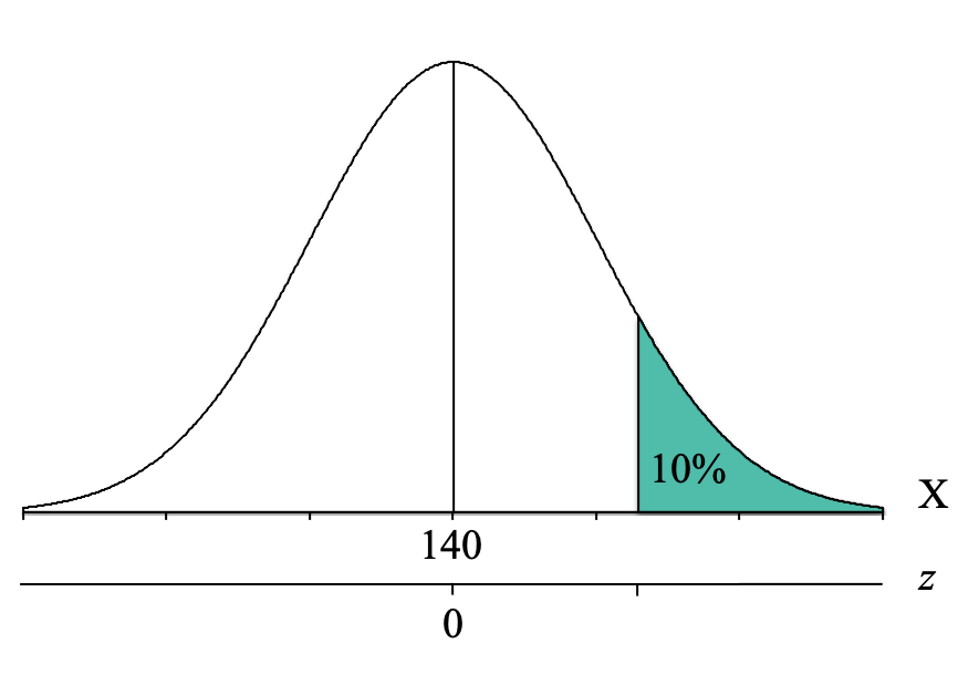
We can now label our distribution graph with the z-score cutoff for the top 10% of z = 1.28:

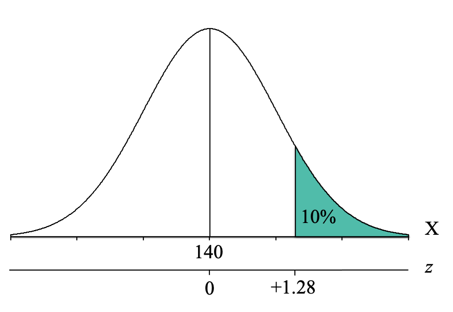
We can see that because the cutoff is above the mean of 0, our z-score cutoff should be positive, and thus is z = +1.28.

Our final step is to convert the z-score cutoff for the top 10% into an individual score (X). To do this, we simply use our z-score formula for individual score that solves for X, and fill in the components:

[latex]X = \mu + z\sigma = 140 + (+1.28)15 = 140 + 19.2 = 159.2[/latex]

We now know that to be in the top 10% on the Multistate Bar Examination, you need to have at least a score of 159.2, which we can now add to our distribution:

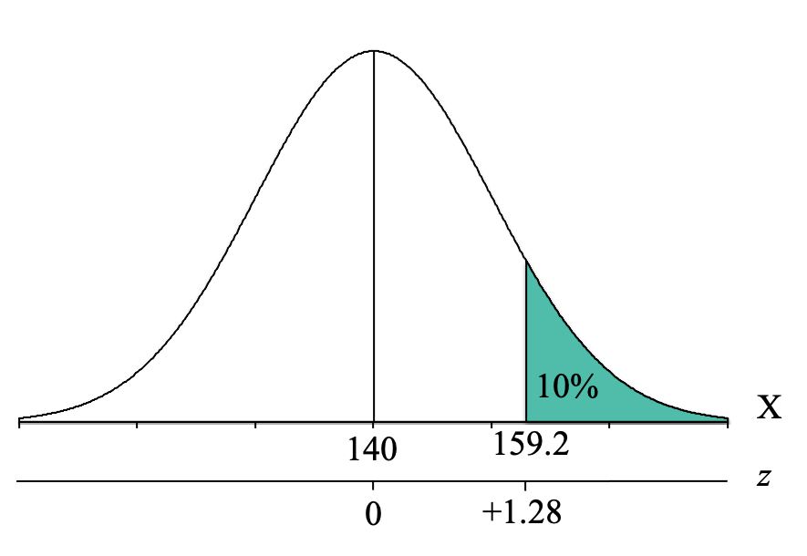
This means that you can screen out any applicants that scored lower than 159.2, and only interview those that scored 159.2 or higher.

Multiple Individual Score (X) Cutoffs from Percentages

Now, imagine you are a teacher and you know that you have a “Goldilocks problem:”

• your teaching pace is too fast for some of your students,
• your teaching pace is too slow for some of your students, and
• your teaching pace is just right for some of your students.

To explore how your class is experienced by different levels of students you decide you want to identify students who are performing extremely poorly and students who are performing extremely well based on the first exam in the class. To identify these students you ask the following question:

To answer this kind of question, we will use the same steps as above, although it will ultimately involve finding two exam score boundaries.

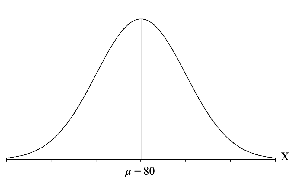
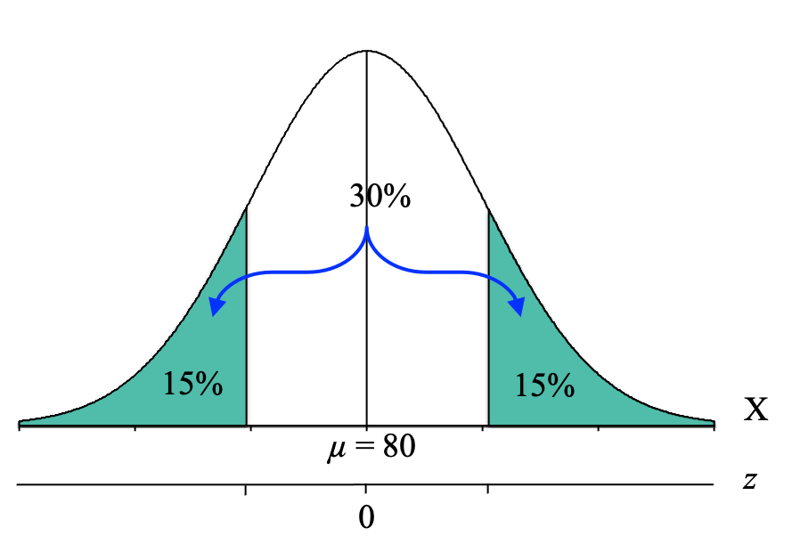
So for our example where we want to know the z-score cutoffs for the extreme 30% of the distribution, we start by drawing the normal distribution and label it with an “X” to indicate that it is a distribution of individual scores on the exam. Then we draw a vertical line in the middle to represent the mean of the exam scores, which is μ = 80. We can label this vertical line with a “μ = 80″ so that we can see from the distribution that most students are scoring near 80, and as you move farther away from 80 in either direction you have fewer students:

Now, we identify the part of the distribution specified in the question, which for our question is the “extreme 30%.” “Extreme” describes the outer edges of the distribution (away from the mean), so we want to shade 30% of our distribution starting from the edges and coming in on both sides until we feel like we have 30% shaded. Because the normal distribution is symmetrical, and we have two extremes (one on the left and one on the right) we will split the percentage of 30% in half, resulting in 15% shaded on each side:

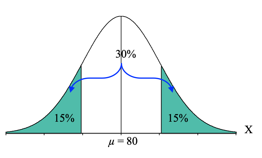
Looking at that picture, the shaded area looks like it has two tails, each shading 15% of the distribution. At this point, we can focus on the upper cutoff (the one that creates the tail of 15% on the right-hand side). We know that this is a tail, so now we just need to convert it to a proportion by dividing by 100, and we get a tail proportion of 0.1500.

We then go to the Unit Normal Table and look in the Tail column.

As you can see in the table, the exact proportion of 0.1500 does not exist in the Tail column. The two closest proportions to 0.1500 are 0.1515 and 0.1492. At this point, we then need to pick the proportion that is the closest to our proportion. By subtracting each of the proportions in the table from our proportion of 0.1500:

[latex]\begin{tabular}[c]{r} 0.1515\\ - 0.1500\\ \hline 0.0015 \end{tabular}[/latex]          [latex]\begin{tabular}{r} 0.1500\\ - 0.1492\\ \hline 0.0008 \end{tabular}[/latex]

We find that the proportion of 0.1492 is closer to .1500, and thus we use the z-score of z = +1.04. Again, because the normal distribution is symmetrical, we don’t need to go through this whole process again to find the z-score cutoff for the lower boundary. It will just be the inverse of the z-score we just located, and thus will be z = -1.04.

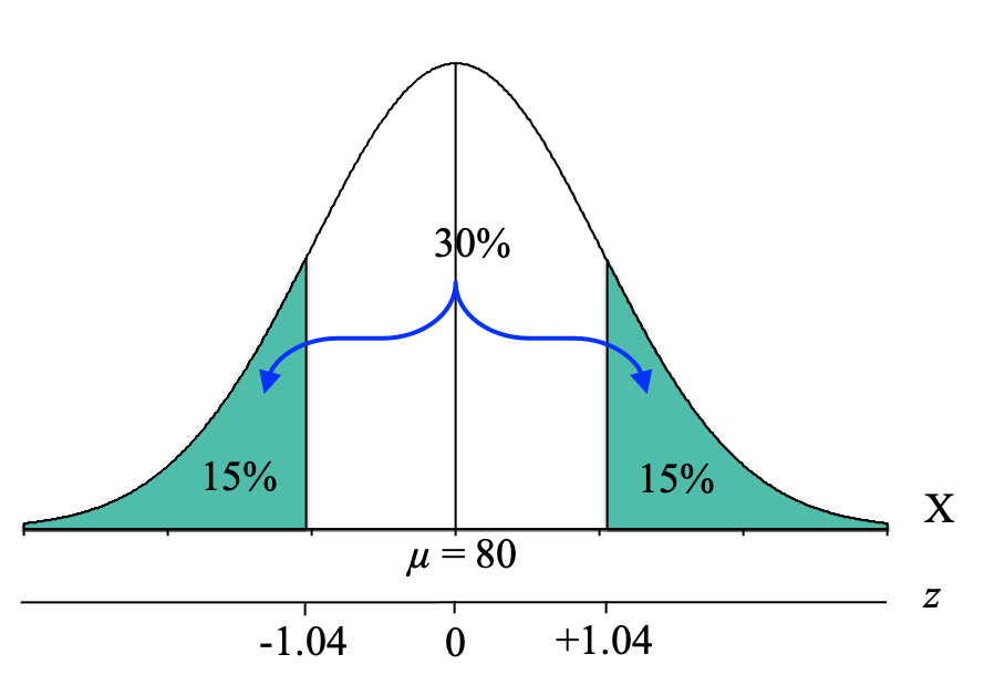
However, it is important to recognize that we are NOT looking for the z-score cutoff for the extreme 30% but rather the Exam 1 score cutoff for the extreme 30%. At this point, it is helpful to add a second axis to the bottom of the distribution graph and label this line with a “z” to indicate that it is the z-score axis. And we can also label the mean with a zero:

We can now label our distribution graph with the z-score cutoff for the extreme 30% of z = -1.04 and z = +1.04:

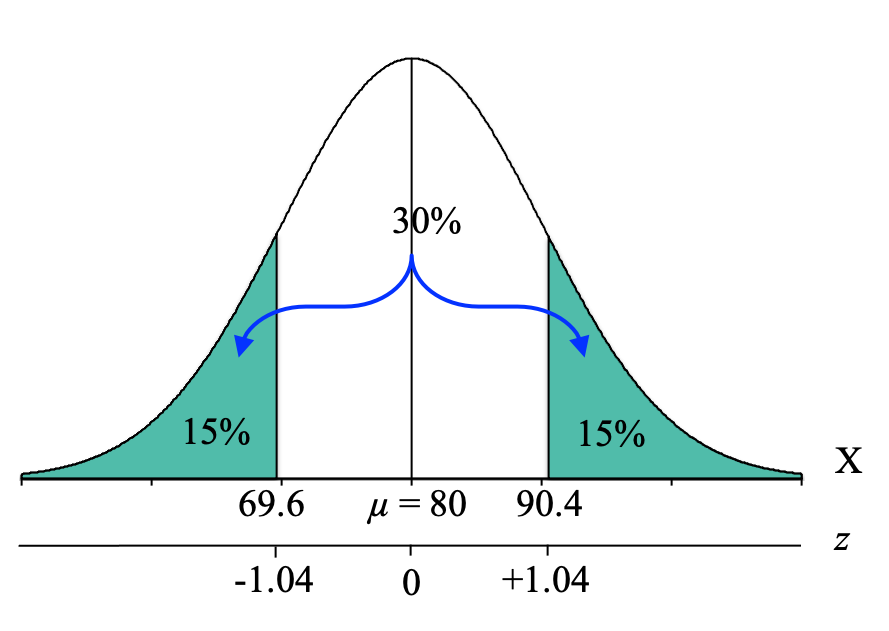
Our final step is to convert the z-score cutoffs for the extreme 30% into an individual scores (X) on Exam 1. To do this, we simply use our z-score formula for individual score that solves for X, and fill in the components:

Lower Boundary: [latex]X = \mu + z\sigma = 80 + (-1.04)10 = 80 - 10.4 = 69.6[/latex]

Upper Boundary: [latex]X = \mu + z\sigma = 80 + (+1.04)10 = 80 + 10.4 = 90.4[/latex]

We now know that the extreme 30% of students on Exam 1 scored below 69.6 or above 90.4:

This means that if you want to find the students who are struggling the most, they are probably the students who scored 69.6 or below on Exam 1. We could then reach out to these students to offer extra help outside of class time. And if you want to find the students who are excelling, they are probably the students who scored 90.4 or higher on Exam 1. We could possibly reach out to them to see if they would be willing to provide tutoring to the students who are struggling.