
7.5 – Finding Proportions or Probabilities from a Sample Mean (M)
In this section, we are going to learn how to find probabilities from a sample mean. To do this, we will use the following steps:
How to find the proportion/probability for a given range of sample means
(Note: Steps 1 through 4 are optional, but help to ground you in the particulars of the question.)
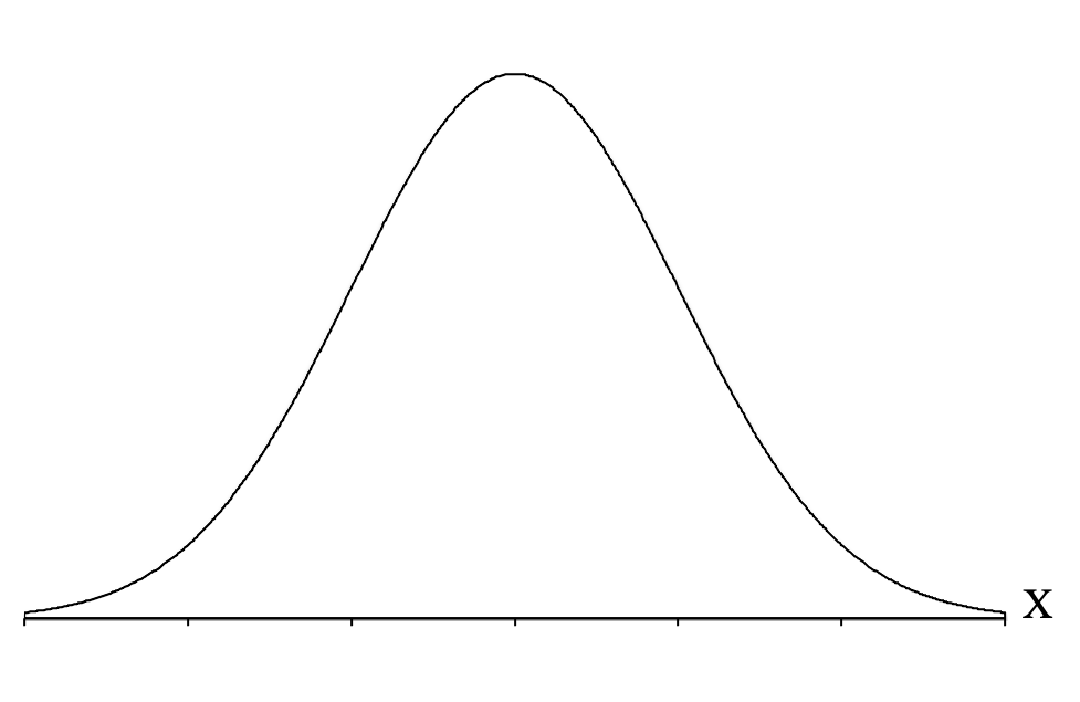
- Draw a picture of the normal distribution curve.
- Label the curve with an X to indicate it is a distribution of individual scores.
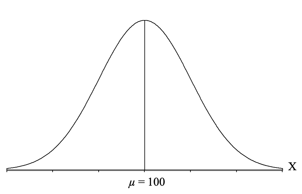
- Draw a vertical line in the middle of the distribution.
- Label this middle line with the population mean, ([latex]\mu[/latex]).
We can now apply the central limit theorem to draw the distribution of sample means of a given sample size and label its mean and standard deviation. This graph represents all of the samples we could get from the population if we were to sample thousands and thousands of samples of the given sample size.
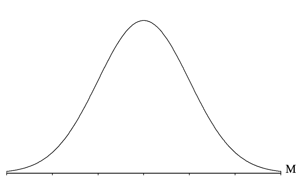
- Draw a second normal distribution curve.
- Label this curve with an M to indicate it is a distribution of sample means.
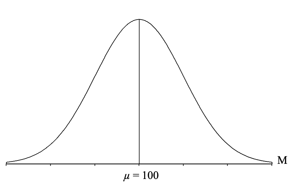
- Draw a verticle line in the middle of the distribution.
- Label this middle line with the population mean, ([latex]\mu[/latex]).
- Draw a horizontal line from the vertical line you just drew to represent the mean to the normal distribution curve on the right.
- Label this horizontal line with the standard error symbol,[latex]\sigma_{\!{_{\!M}}}[/latex].
- Calculate the standard error using the formula: [latex]\sigma_{\!{_{\!M}}} = \frac{\sigma}{\sqrt n}[/latex].
We now will locate a range of these sample means based on the question we are attempting to answer.
- Locate the sample mean on the curve (approximately) and label it with a vertical line.
- Shade the appropriate part of the distribution (e.g., above the sample mean, below the sample mean, between the population mean and the sample mean).
- Look at the shaded chunk and decide if it is a body, a tail, or a slice.
- Calculate the z-score for the sample mean using the formula:
[latex]z = \frac{M - \mu}{\sigma_{_{\!M}}}[/latex] - Create a second x-axis below the individual-score axis, label the middle vertical line as z = 0, and label the vertical line for the real-world score as the z-score you calculated from the previous step.
- Look up your z-score in the first column of the Unit Normal Table.
- Then go across that row to the appropriate column (Body, Tail, or Slice) from step 14 to get your answer.
Let’s say we want to answer the question:
Being “normally distributed,” tells us that if you were to create a graph of the IQ scores of all the individuals in a population, it would form a normal distribution which means that most individuals tend to score near the mean, and as you get farther from the mean, in either direction, you get fewer and fewer people. We also know that the average score for individuals on the IQ test is 100, and individuals in the population deviate from that mean by an average of 15 points.
So now we can follow our steps and draw a normal distribution curve and label it on the side with an X to indicate that it is a distribution of individual scores:
Next, we draw a vertical line in the middle of the distribution and label it with the mean for IQ tests (which is given to us in the question) of μ = 100:
Next, we need to apply the central limit theorem and draw a distribution of all the sample means we could get for a sample size of n = 25 (because that is the sample size from our question). The central limit theorem essentially predicts what the distribution of sample means would look like for thousands and thousands of samples of 25 people.
The first thing the central limit theorem predicts is the shape of the distribution of sample means. Remember, that the distribution of sample means will form a normal distribution if you meet either of these two conditions:
- You are sampling from a population that is normally distributed.
- Your sample size is at least n = 30.
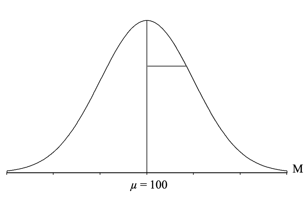
We meet the first condition because IQ scores in the population are normally distributed, so our distribution of sample means will be normally distributed. Thus, we draw another normal distribution, but this time we label it with an M to indicate that it is a distribution of sample means:
Next, we draw a vertical line in the middle of the distribution and label it with the mean of all the sample means ([latex]\mu_{_{\!M}}[/latex]), which as we know from the central limit theorem is going to be equal to the population mean (which is given to us in the question) of μ = 100:
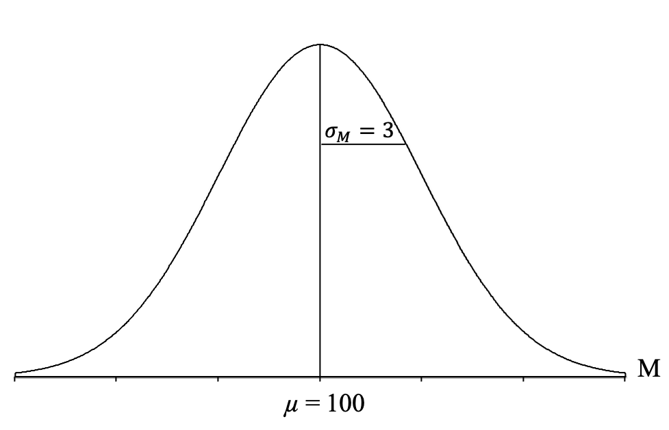
Next, we draw a horizontal line from the vertical line representing the mean to the curve on the right. This will depict the standard deviation of all of the sample means in this distribution:
The second thing that the central limit theorem tells us is that this standard deviation of all of the sample means can be calculated using the formula for the standard error ([latex]\sigma_{\!{_{\!M}}}[/latex]), so we can plug in the population standard deviation (σ) and sample size (n) given to us in the question and calculate the standard error:
[latex]\sigma_{\!{_{\!M}}} = \frac{\sigma}{\sqrt n} = \frac{15}{\sqrt 25} = \frac{15}{5} = 3[/latex]
We can then add the standard error to our graph:
It can be very helpful to take a moment here and try to understand what this distribution depicts. It is a theoretical distribution of thousands and thousands of sample means, each coming from samples of n = 25 people, taken from the population of individual IQ scores (that are normally distributed, have a mean of μ = 100, and a standard deviation of σ = 15). These sample means form a normal distribution, have a mean of 100, and a standard deviation of 3, which indicates that most of the sample means are centering around 100, and deviate from 100 by about 3 points on average, with some above and some below 100. Many of the sample means tend to be near 100, and as you get farther from 100, in either direction, you get fewer and fewer sample means.
It is also worth noting that is a theoretical distribution because we applied the central limit theorem to create it. We didn't have to take thousands and thousands of samples to create it. If we had, it would look very very close to this, but we don't need to go through all that work and can instead just do the calculations and draw it.
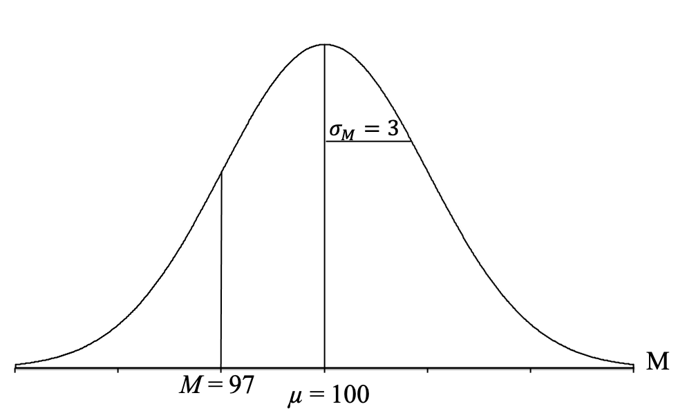
Now, let's return to answering our question. Our next step is to locate the sample mean of M = 97 on the graph. Since the sample mean of 97 is below the mean of 100, we can put a vertical line to the left of the mean. It doesn’t matter exactly how far we put the line above the mean because only using it to determine what proportion column (body, tail, or slice) to use. For our computer-generated graph, you can use the tick marks on the bottom axis to help because each of them represents a standard deviation from the mean:
To find the probability of getting sample means higher than 97, we want to know the proportion (remember, proportion = probability) of the normal distribution that lies above (or is greater than) the sample mean of M = 97. Thus, we shade the part of the distribution that includes all the sample means that are higher than 97 (or to the right of the vertical line at M = 97). In other words, we want the following proportion of P (M > 97):
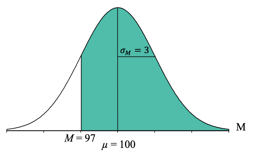
Looking at that picture, we see that the shaded area is a “body,” which tells us that we will find the proportion/probability in the Tail column of the Unit Normal Table.
However, the cutoff point for that body is not a z-score but is instead sample mean (M). Thus, we need to calculate the z-score for the sample mean of M = 97. To do that, we simply use the z-score formula that solves for z:
[latex]z = \frac{M - \mu}{\sigma_{_{\!M}}}[/latex]
When we plug in everything we were given and calculated:
- M = 97 (given)
- μ = 100 (given)
- [latex]\sigma_{\!{_{\!M}}} = 3[/latex] (calculated)
Now we plug it into our z-score formula for sample means:
[latex]z = \frac{X - \mu}{\sigma} = \frac {97 - 100}{3} = \frac{-3}{3} = -1.00[/latex]
We find that the sample mean of 97 corresponds to a z-score of -1.00. In other words, the sample mean of 97 is one standard deviation, or standard error, below the mean of 100.
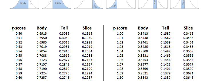
Next, we go to the Unit Normal Table and look for our z-score of z = -1.00 in the z-score column. An important thing to note is that z-scores in the Unit Normal Table are all positive, but we know that normal distributions are symmetrical so the body for z = -1.00 is the same as the body for z = +1.00. When we look across the z = 1.00 row until we come to the Body column, we find a proportion of P (z > -1.00) = 0.8413, or 84.13% of the normal distribution lies above a z-score of z = -1.00.
Because that z-score of -1.00 corresponds to a sample mean of 97, we know the proportion of sample means (of a sample size of n = 25) above 97 on an IQ test is 0.8413, or 84.13% of sample means (of a sample size of n = 25) will be above 97 on an IQ test.
And then, because proportion equals probability, we now know that the probability of a sample of n = 25 individuals having an IQ score average greater than 97 is 0.8413.
Another way of putting it is that if you were to randomly grab 25 people, have them take a standardized IQ test, and then average their scores, there is a 84.13% chance that those 25 people will have an average IQ score above 120.

Feedback/Errata