
6.6 – Finding Z-scores from Proportions or Percentages
We can also use the Unit Normal Table to find z-scores if we know a particular proportion. For example, let’s say we wanted to find the z-score that serves as the cutoff point for the top 30%. To do this, we follow very similar steps as before:
How to find a z-score for a given percentage
- Draw a picture of the normal distribution curve.
- Draw a vertical line in the middle of the distribution.
- Label this middle line with a z = 0.
- Identify the part of the distribution specified in the question (e.g., top, bottom, middle, extreme) and shade the specified percentage (e.g., top 25% means about 1/4 of the shape should be shaded on the right-hand side).
- Look at the shaded portion and decide if it is a body, a tail, or a slice.
- Convert the percentage from the question into a proportion by dividing by 100.
- Look up your proportion in the appropriate column of the Unit Normal Table (Body, Tail, or Slice).
- Then go across that row to the z-score column to get the z-score cutoff answer.
- Label the cutoff on the distribution graph to help you determine if it needs to be a positive or negative z-score.
From a Percentage to a z-score
So for our example above, we want to answer the following:
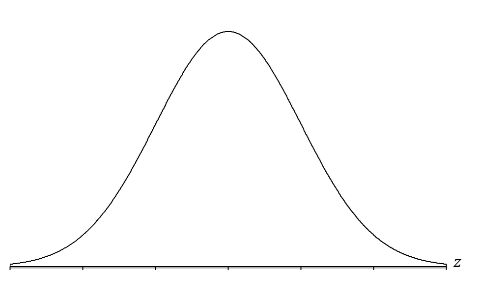
We start by drawing the normal distribution and labeling it with a "z" on the right, to indicate that it is a distribution of z-scores:
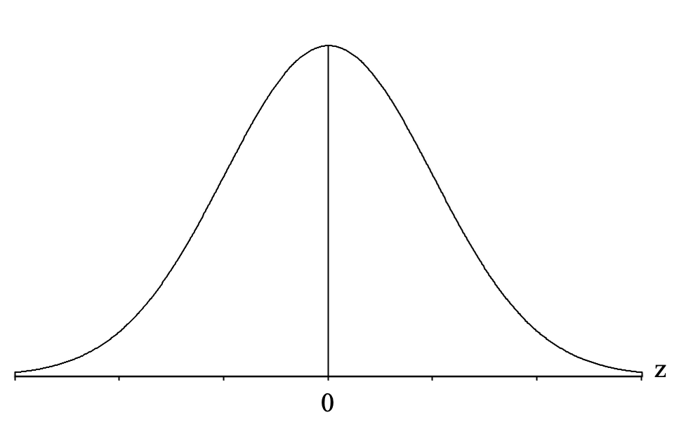
Then we draw a vertical line in the middle to represent the mean. We can label this vertical line with a "0" because the mean for z-scores is always zero:
Now, we identify the part of the distribution specified in the question, which for our question is the "top 30%." "Top" means on the right-hand side of the distribution because that is where the higher, or "top," scores are located (remember that the x-axis is a number line and higher scores are to the right). So we want to shade 30% of our distribution starting from the right-hand side:
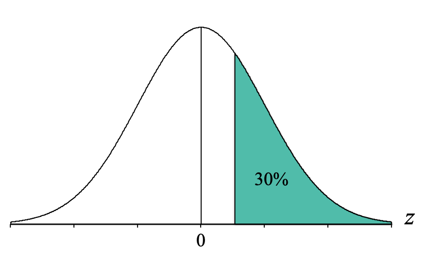
At this point, it doesn’t matter if it is exactly 30% shaded because we only are using it to determine what proportion column (body, tail, or slice) to use. Looking at that picture, we can see that the shaded area is a “tail.” We then go to the Unit Normal Table and look in the Tail column for our percentage. However, the Unit Normal Table displays proportions not percentages. Thus, we need to convert our percentage to a proportion. To convert our percentage of 30% to a proportion we simply divide it by 100. Thus, we look for the proportion of 0.3000 (make sure to use four decimal places because the proportions in our Unit Normal Table go to four decimal places).
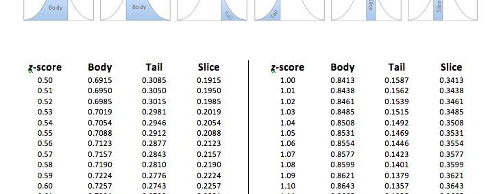
As you can see in the table, the exact proportion of 0.3000 does not exist in the Tail column. The two closest proportions to 0.3000 are 0.3015 and 0.2981. At this point, we then pick the proportion that is the closest to our proportion. By subtracting each of the proportions in the table from our proportion of 0.3000 we find that the proportion of 0.3015 is 0.0015 or fifteen ten thousandths away, while the proportion of 0.2981 is 0.0019 or nineteen ten thousandths away:
[latex]\begin{tabular}[c]{r} 0.3015\\ - 0.3000\\ \hline 0.0015 \end{tabular}[/latex] [latex]\begin{tabular}{r} 0.3000\\ - 0.2981\\ \hline 0.0019 \end{tabular}[/latex]
Thus, the proportion of 0.3015 is a little bit closer. So now we use the proportion of 0.3015, and simply go across that row to the z-score column to find the z-score cutoff. We have now determined that the z-score cutoff for the top 30% is at z = 0.52.
We should now label our distribution graph with the z-score cutoff:
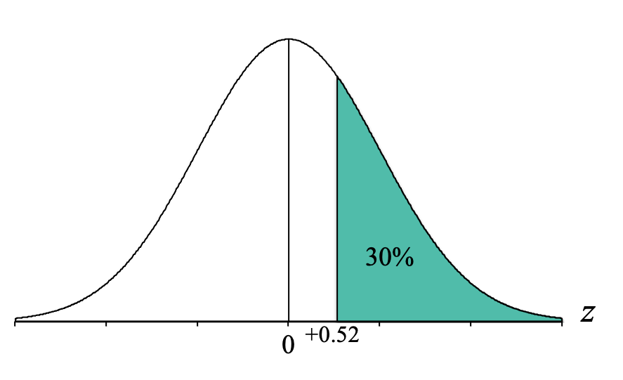
We can see that because the cutoff is above the mean of 0, our z-score cutoff should be positive, and thus is z = +0.52.
Determining if the z-score is Positive or Negative
One thing to be careful about when searching for z-score cutoffs is that the Unit Normal Table does not include any negative z-scores. This is where your drawing will be very important.
Let’s say, for example, that you want to answer this question:
To do this, we follow the same steps as above. So for our example where we want to know the z-score cutoff for the top 75% of the distribution, we start by drawing the normal distribution:
Then we draw a vertical line in the middle to represent the mean. We can label this vertical line with a "0" because the mean for z-scores is always zero:
Now, we identify the part of the distribution specified in the question, which for our question is the "bottom 75%." "Bottom" means on the left-hand side of the distribution because that is where the lower, or "bottom," scores are located (remember that the x-axis is a number line and lower scores are to the left). So we want to shade 75% of our distribution starting from the left-hand side:
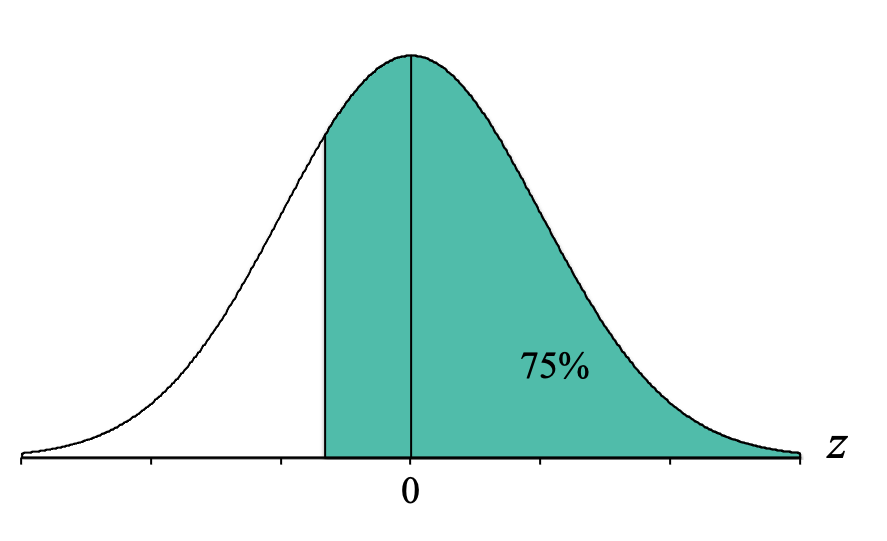
Looking at that picture, we can see that the shaded area is a “body.” We then go to the Unit Normal Table and look in the Tail column. To convert our percentage of 75% to a proportion we simply divide it by 100. Thus, we look for the proportion of 0.7500 (make sure to use four decimal places because the proportions in our Unit Normal Table go to four decimal places, thus instead of 0.75 we will use 0.7500).
As you can see in the table, the exact proportion of 0.7500 does not exist in the Body column. The two closest proportions to 0.7500 are 0.7486 and 0.7517. At this point, we then need to pick the proportion that is the closest to our proportion. By subtracting each of the proportions in the table from our proportion of 0.7500...
[latex]\begin{tabular}[c]{r} 0.7500\\ - 0.7486\\ \hline 0.0014 \end{tabular}[/latex] [latex]\begin{tabular}{r} 0.7517\\ - 0.7500\\ \hline 0.0017 \end{tabular}[/latex]
we find that the proportion of 0.7486 is 0.0014 or fourteen ten-thousandths away, while the proportion of 0.7517 is 0.0017 or seventeen ten-thousandths away. Thus, the proportion of 0.7486 is a little bit closer to our desired proportion of 0.7500.
So now we use the proportion of 0.7486, and simply go across that row to the z-score column and we see that the z-score cutoff for a body of 75% is closest to a z = 0.67.
We should now label our distribution graph with the z-score cutoff:

When we do this, we can see that because the cutoff is below the mean of 0, our z-score cutoff should be negative, and thus is z = -0.67. This is where drawing the pictures is super helpful because the Unit Normal Table can't tell you if the z-score should be positive or negative because it only uses positive z-scores.
Multiple z-scores From Percentages
One other type of percentage question we will want to be able to answer involves "middle" or "extreme" percentages, which result in more than one cutoff score. Consider the following question:
To answer this kind of question, we will use the same steps as above, although it will ultimately involve finding two z-score boundaries. We may also have to get creative when determining what type of shape to look up in the Unit Normal Table (body, tail, or slice).
So for our example where we want to know the z-score cutoffs for the middle 90% of the distribution, we start by drawing the normal distribution:
Then we draw a vertical line in the middle to represent the mean. We can label this vertical line with a "0" because the mean for z-scores is always zero:
Now, we identify the part of the distribution specified in the question, which for our question is the "middle 90%." "Middle" describes the center of the distribution (near the mean of zero), so we want to shade 90% of our distribution starting from the middle and extending equally to the left and right:
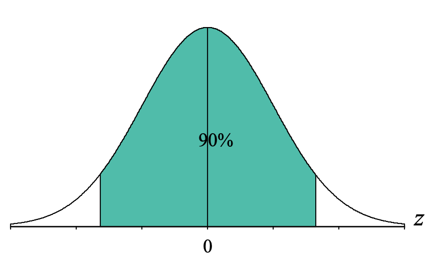
Looking at that picture, the shaded area does not look exactly like a body, a tail, or a slice, so this is where we have to get a little creative. Because the Unit Normal Table only has proportion columns for the body, tail, or slice, we need to convert our middle 90% into a percentage that is either a body tail or slice.
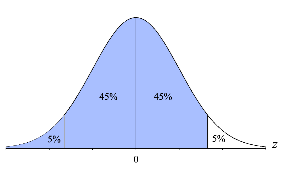
One thing to remember is that normal distributions are symmetrical, so we can break up the 90% into two halves of 45% (just divide the percent by two: [latex]\frac{90}{2} = 45[/latex]. We also know that if there is 90% shaded in the middle, that means that there is 10% that is not shaded, and again, that 10% can be divided in half, resulting in 5% not shaded on either side. Thus, we get the following distribution:
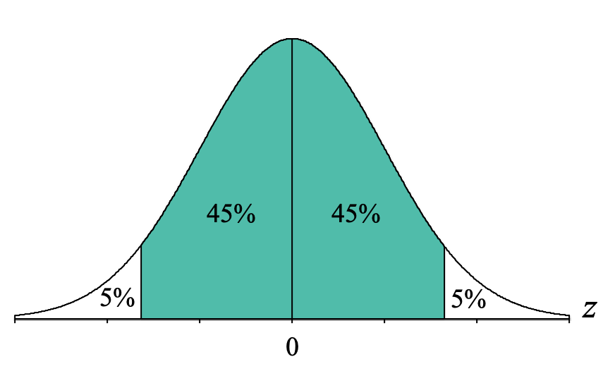
Hopefully, this helps us come up with possible paths to identify a body, tail, or slice. To help the process along, it can be useful to focus on that upper boundary for the middle 90%:
![]()
If we want to determine the percentages for the different proportion columns in the Unit Normal Table, we can do the following:
- Body: Add all the percentages to the left of that line: 5% + 45% + 45% = 95%
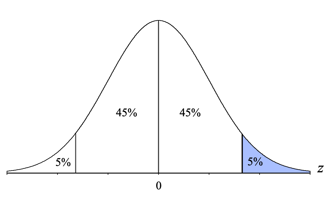
- Tail: Use the percentage to the right of that line: 5%
- Slice: Use the percentage between that line and the mean: 45%
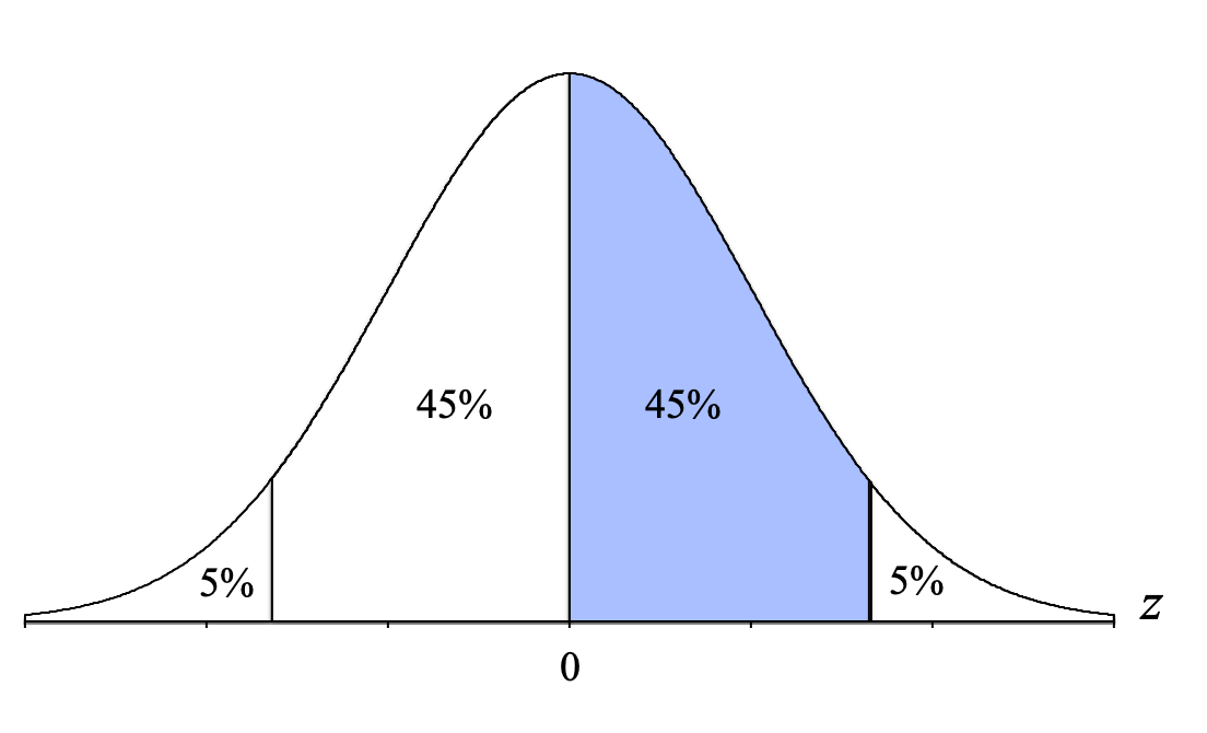
Ultimately, you can use any of these three solutions because they will all result in the same answer. (Note: It's typically a good idea to choose whichever one makes the most sense to you.) Let's use the slice option this time.
We then go to the Unit Normal Table and look in the Slice column. To convert our slice percentage of 45% to a proportion we simply divide it by 100. Thus, we look for the proportion of 0.4500 (make sure to use four decimal places because the proportions in our Unit Normal Table go to four decimal places, thus instead of 0.45 we will use 0.4500).
As you can see in the table, the exact proportion of 0.4500 does not exist in the Slice column. The two closest proportions to 0.4500 are 0.4495 and 0.4505. At this point, we then need to pick the proportion that is the closest to our proportion. By subtracting each of the proportions in the table from our proportion of 0.4500:
0.4500 - 0.4495 = 0.0005
0.4505 - 0.4500 = 0.0005
We find that neither proportion is closer because they are both 0.0005 or 5 ten-thousandths away. When a situation like this happens, when our proportion is equidistant from two proportions in the Unit Normal Table, we will choose the higher of the two z-scores. The reason for this will make more sense in the future and has to do with being careful to not exceed a specified probability when we are using hypothesis testing and inferential statistics.
So because the z-scores corresponding to our two proportions are 1.64 and 1.65, we will use the higher of the two as our cutoff. So now we know that the z-score boundary (on the upper end, for now) is z = +1.65.
Thankfully, because the normal distribution is symmetrical, we don't need to go through this whole process again to find the z-score cutoff for the lower boundary. It will just be the inverse of the z-score we just located, and thus will be z = -1.65. We can now label our distribution graph with both z-score cutoffs:
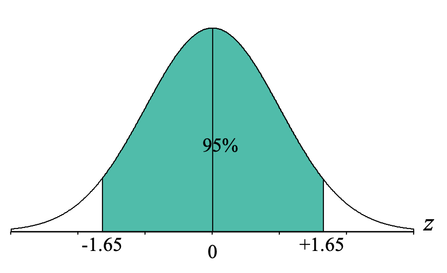
We can now interpret this to mean that 95% of z-scores from a normal distribution fall between z = -1.65 and z = +1.65.
One last thing. What if we wanted to answer this related question?
The word "extreme" indicates that we are looking for scores that exceed or strongly differ from the usual or normal. In a normal distribution, the usual or normal scores (in other words, scores that happen frequently) are the scores in the middle. We can see that the normal curve has a high frequency around the mean. Thus, the "extreme" or unusual scores are out in the sides to the left or right.
To graph the extreme 10%, we start at both the extreme left and extreme right and come in until we have shaded about 10% of the distribution:

And again, because the normal distribution is symmetrical, we can split the 10% into equal halves of 5%, and we end up with:

And from here, hopefully, we can see that if we focus on that upper boundary, it is a tail of 5%. We can then convert it to a proportion of 0.0500 by dividing 5% by 100, look in the Tail column for 0.0500. We will find that it is equidistant from the proportions of 0.0495 and 0.0505, so we go with the higher z-score of z = +1.65. And because it's symmetrical, we know that the cutoff for that bottom 5% is z = -1.65:
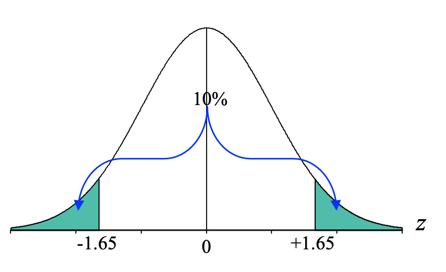
This tells us that only 10% of scores are below z = -1.65 or above z = +1.65. In other words, these are rare or unusually different scores. And this will come in handy later on when we try to answer research questions.

Feedback/Errata