7.3 – The Central Limit Theorem

As we saw in the previous section, when we take a sample from a population there is going to be a good amount of sampling error when our sample is not perfectly representative of the population (which is most of the time). While this would seem to make using samples to try to understand things about a population a pointless endeavor, it turns out that we can identify a pattern to how samples and ultimately sampling error tend to work. We can then take this predictable pattern into account when we use the sample to try to understand something about the population, such as using a sample mean to guess at the population mean.

Statisticians explain these patterns in a concept in probability theory called the Central Limit Theorem. The Central Limit Theorem, for our purposes, states that if you take samples of the same sample size (n) from a population (with a mean of μ and s standard deviation of σ) and calculate each sample’s sample mean (M), then the distribution of a sufficiently large number of these sample means will approach a normal distribution as n approaches infinity (even if the original population is not normally distributed), have an overall mean equal to the population mean ([latex]\mu_{_{\!M}} = \mu[/latex]), and have an overall standard deviation equal to the standard error ([latex]\sigma_{\!{_{\!M}}} = \frac{\sigma}{\sqrt n}[/latex]).

For most students, this theory is complex and difficult to understand. Thankfully, it is not necessary to memorize the theory but instead be able to apply it. Thus, we will examine the theory in order to extract the important applications for our purposes. (It is also worth noting that the term “central limit theorem” is actually associated with a number of different statements regarding the convergence of probability distributions in probability theory.^[1]

Let’s begin with the basic setup for how we will use the central limit theorem. Let’s say we want to measure something in a group of individuals but don’t have the time or resources to measure everyone so we can only use a sub-group of those individuals. For example, imagine we want to know the average high school grade point average (HS GPA) of community college students. It would be nearly impossible to ask all currently enrolled community college students about their HS GPA, so instead, we will just poll a subset of 100 randomly-selected community college students. Hopefully, you recognize this as the typical setup of a research study where we are going to use a sample to describe something about a population.

Now it is likely that the average HS GPA of this sample of 100 community college students would not be exactly the same as the HS GPA of all community college students. Because of sampling error, we might sample a group that has a higher or lower average HS GPA. And we aren’t going to know which direction the error goes. It seems a bit pointless.

Imagine, though, that we then take one thousand more samples of 100 randomly-selected community colleges and calculate the sample mean for each of those one thousand samples. We would now have one thousand and one sample means (our original sample mean and the new one thousand we collected just now). Again, the average HS GPA of each of these one thousand samples (sample means, M) are not likely to be exactly the same as the HS GPA of all community college student (the population mean, μ). Because of sampling error, some might have higher average HS GPA’s and some might have lower average HS GPA’s (and some will have no sampling error and will actually equal the population mean). And this is where the central limit theorem can help us.

The central limit theorem ultimately predicts 3 things about these one thousand and one sample means:

1. The shape of the distribution of sample means will be approximately normal, as n approaches infinity.
2. The mean of all these sample means will equal the population mean, [latex]\mu_{_{\!M}} = \mu[/latex].
3. The standard deviation of all these sample means can be calculated as the standard error which is equal to: [latex]\sigma_{\!{_{\!M}}} = \frac{\sigma}{\sqrt n}[/latex].

So this can tell us what our one thousand and one sample means will look like (without ever having to actually go through the process of sampling one thousand and one samples!):

1. They will form a roughly normal, or bell-shaped, distribution.
2. The mean of all these HS GPA sample means will be roughly the same as the population HS GPA.
3. The standard deviation of these sample means can be calculated as the standard error, equal to: [latex]\sigma_{\!{_{\!M}}} = \frac{\sigma}{\sqrt n}[/latex]

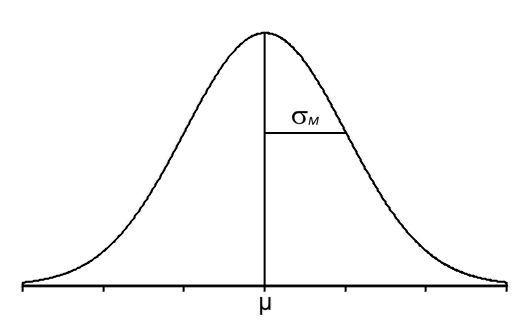
Think of the above graph as a pile of sample means stacked on top of each other:

Think of each box in the distribution above as representing a single sample mean (M) measured from an individual sample of a given sample size (n) taken from a given population.

Then, by looking at hundreds of individual sample means, we can now see that there is a pattern to the results. There are a lot of sample means near the population mean of μ because the curve has a high frequency. As you get farther from the population mean, you get fewer and fewer sample means, and the frequency gets lower.

Hopefully, you will also notice that this distribution looks similar to our chapters on the z-score and probability because it is a Normal Distribution, which is what the Central Limit Theorem predicts (if we meet certain criteria). Thus, like in the last chapter, if we were to shade part of this distribution, we could use the Unit Normal Table to look up proportions/probabilities as long as we know the z-score or z-scores that form the boundary or boundaries of the shaded area.

And that brings us to the z-score formulas for sample means.