Section 5.4: The Sampling Distribution of a Percentage
To determine how a sample percentage compares to the true population percentage, Statisticians looked at what would happen if we knew the true value of the percent we were looking for and how much error we could expect based on the sample size. In what follows, we will do the same.
Arizona’s currently has 3,632,377 registered voters. This is a lot of people! Collecting data is expensive and requires a lot of time and effort so we don’t want to survey all of them. The good news is, when the population is sufficiently large we do not need to consider the size of the population when choosing a size of a sample. Meaning, we don’t need 10% of the population (363,238) or some amount that depends on the size of the population. We will use statistical theorems and results that are independent of the population size.
I know the phrase sufficiently large is somewhat cryptic and vague. A good rule of thumb is that the sample should have at least 5 results for each outcome. In our example, this would mean that in our sample, at least 5 people should respond in favor of the proposition and at least 5 people should respond against the proposition.
I. The Sampling Distribution of a Proportion (or Percentage)
For argument’s sake, we will assume that we know the true percentage of people that will vote in favor of the proposition. Let’s say that this percent is 52%. In statistics, this percent is frequently called a proportion where we think of 52% as a fraction of the number of votes in favor of the proposition over the total number of votes [latex]\frac{52}{100}[/latex]. (Note that in math we call this a ratio or fraction, and a proportion is a statement that two ratios are equal. So the terminology differs in this context.) We typically use the letter p to denote the population proportion. When we take a sample from a population to estimate the population percentage p, we label the resulting sample percentage 𝑝̂ pronounced “p hat”.
So if we assume 52% of the voters vote in favor of the proposition, or p = 52% what can we expect a sample of this population to look like? First let’s start with a really small sample size of 3. We denote the sample size of a survey with the letter n. So here, n = 3.
If we sample three people, we can get 0, 1, 2, or 3 yes votes in our sample. The table below shows how this may happen with “0” representing a vote of No and “1” representing a vote of Yes.
| Number of Yes Votes | Arrangement of Yes Votes in Sample | Proportion or Percentage of Yes Votes |
| Zero Yes votes | 0 0 0 | 𝑝̂ = [latex]\frac{0}{3}[/latex] = 0% |
| One Yes vote | 1 0 0 or 0 1 0 or 0 0 1 | 𝑝̂ = [latex]\frac{1}{3}[/latex] ≈ 33.3% |
| Two Yes votes | 1 1 0 or 0 1 1 or 1 0 1 | 𝑝̂ = [latex]\frac{2}{3}[/latex] = 66.7% |
| Three Yes votes | 1 1 1 | 𝑝̂ = [latex]\frac{3}{3}[/latex] = 100% |
Observations: There are a few important things to notice from this table.
1) Each of the estimates for the percentage of voters who will vote yes, 𝑝̂ , is far from the true value. Recall the true value is p = 52%. A sample size of 3 is not useful!
2) We are more likely to get a sample with 1 or 2 yes votes than 0 or 3 votes (3 ways to get 1or 2 yes votes as opposed to 1 way to get 0 or 3 yes votes)
3) Even though there are an equal number of ways to get 1 or 2 yes votes, we are more likely to get 2 yes votes than 1 yes vote since the chance of a yes vote is 52% and the chance of a no vote is 48%.
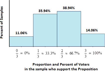
The true chance or probability of getting each of these samples in displayed in the histogram below. The horizontal axis represents the proportion or percentage of yes votes in the sample. The vertical axis represents the percent of all possible samples that would give us the sample on the horizontal axis. (The mathematics of how these chances are computed are beyond the scope of the course, but you may look them up by researching Binomial Distributions or probabilities if you are interested.)

Interpretation: The true percent of population: p = 52% Sample Size: n = 3
If we collect a sample size of 3 from a population with a true population percent of 52%
11.06% of the time, the sample proportion, 𝑝̂ , will equal 0%.
35.94% of the time, the sample proportion, 𝑝̂ , will equal 33.33%.
38.94% of the time, the sample proportion, 𝑝̂ , will equal 66.67%.
14.06% of the time, the sample proportion, 𝑝̂ , will equal 100%.
So we know that a sample size of 3 isn’t useful. What sample size would give us a good or better estimate? We will look at sample sizes of increasing sizes and look for patterns in the distributions.
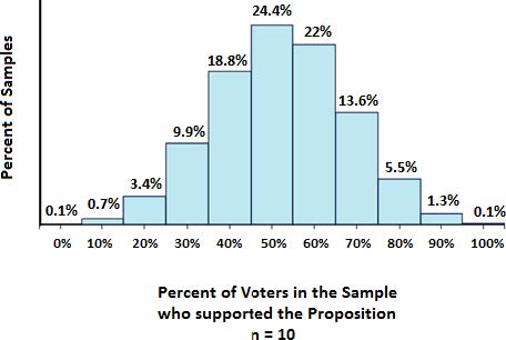
Sample Size = 10
The histogram below shows the distribution of sample percentages for a sample size of 10. The mode percentage is 50% which is closest to the true value of 52%, but with this sample size, we still could not even obtain the true value from the sample.

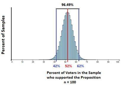
Sample Size = 100
The histogram below shows the distribution of sample percentages for a sample size of 100. Notice that the distribution is narrowing and centered at the true population percentage of 52%. Listing all of the percentages for the different percent of voters from the sample who support the proposition is no longer useful. However, notice that 96.49% of the possible samples will give a sample percent between 42% and 62% which is the true population percentage plus or minus 10%.

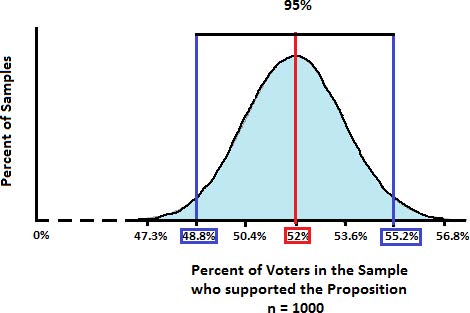
Sample Size = 1000
The next histogram shows the distribution of sample percentages for a sample size of 1000. Notice that as the sample size increases, more of the sample percentages are close to the true value of the population percentage. The histogram itself may not appear narrower because the scaling of the horizontal axis changed to focus in on the values where most of the sample percentages lie. Also notice there doesn’t appear to be any histogram bars. These rectangles have such a small width that the distribution looks smooth. The larger the sample size, the smoother the distribution becomes. In fact, it can be closely approximated by a Normal Distribution or Bell Curve that you may have heard or learned about in prior courses.

II. 95% Confidence Intervals and the Margin of Error
We noticed that as the sample size increased from 0 to 10 to 100 and then to 1000, more of the sample percentages lie “close” to the true value of the population proportion. Now we would like to quantify this closeness. First we will start with a definition and then we will state a formula that quantifies the precision.
Definition: A 95% Confidence Interval for the population percentage is an interval of values centered at the true population percentage that includes 95% of all possible sample percentages. It depends on the true population percentage and the sample size.
Interpretation: For the last example with n = 1000 and p = 52%, the 95% Confidence Interval is (48.8%, 55.2%). We can state that for all possible samples of size 1000, 95 out of 100 will have a sample percentage between 48.8% and 55.2%.
Note: We could use other percentages for the Confidence Interval. Some popular ones are 99%, and 90%. We will use 95% for convenience and because it is frequently used in practice.
Definition: The Margin of Error for a population proportion with a 95% Confidence Interval is the difference between the true population proportion and either end point of the 95% Confidence Interval. Equivalently, the Margin of Error (or MOE) is half the distance of the length of the 95% Confidence Interval.
Example: For the last example with n = 1000 and p = 52%, the 95% Confidence Interval is (48.8%, 55.2%). The Margin of Error can be computed in any of the following ways:
55.2% - 52% = 3.2% or 52% - 48.8% = 3.2% or [latex]\frac{55.2\%~-~48.8\%}{2}[/latex] = [latex]\frac{6.4\%}{2}[/latex] = 3.2%
III. Conservative Estimate for the Margin of Error for a 95% Confidence Interval
There is a formula to compute the Margin of Error based on the population proportion p and the sample size n. We can simplify it greatly if we use a conservative estimate that only uses the sample size n. Meaning the Margin of Error we compute will be slightly larger than the actual Margin of Error, but since this is erring on the side of caution, it is worth the simplification.
A conservative estimate of the MOE for a 95% Confidence Interval with sample size n is:
MOE = [latex]\frac{1}{\sqrt{n}}[/latex]
Since we report this as percentage, we can use:
MOE = [latex]\frac{1}{\sqrt{n}}[/latex] • 100%
Example 16: For the last example, n = 1000. So the MOE = [latex]\frac{1}{\sqrt{1000}}[/latex] • 100% ≈ 3.2% (rounded to one decimal place). Typically, we will use this formula to find the 95% Confidence Interval rather than creating a histogram.
The formula for the 95% Confidence Interval based on p and the MOE is (p − MOE, p + MOE).
Which for this example is (52% − 3.2%, 52% + 3.2%) = (48.8%, 55.2%)
Example 17: Worked Example - MOE and 95% Confidence Interval for a Population %
The value of a population percent is p = 63%. For sample sizes of n = 1357, find the MOE and 95% Confidence Interval and interpret the CI. Round to two decimals as needed.
Solution: MOE = [latex]\frac{1}{\sqrt{1357}}[/latex] • 100% ≈ 2.71%
The 95% CI is (63% − 2.71%, 63% + 2.71%) = (60.29%, 65.71%)
95 out of 100 samples of size n = 1357 will have sample percentages that lie between 60.29% and 65.71%.
1) As the sample size increases, more samples will have a sample percentage close to the true value.
2) We can conservatively estimate that 95% of the sample percentages with population percentage p and sample size n will lie in the interval (𝑝 − [latex]\frac{1}{\sqrt{n}}[/latex] , 𝑝 + [latex]\frac{1}{\sqrt{n}}[/latex]) We call this the 95% Confidence Interval for the sampling distribution of the percentage.
3) The value [latex]\frac{1}{\sqrt{n}}[/latex] written as a percentage is a conservative estimate for the Margin of Error of a sample percentage using a 95% confidence interval. The Margin of Error is an estimate of the sampling error that occurs when we use a sample to estimate a population.
4) Sampling error is the name for the variability of possible sample percentages. It is not an “error” that was made by the pollster, but a consequence of taking a sample from a population. It cannot be avoided when taking a sample, but can be minimized by taking a larger sample.
