
6.3: Newton’s Laws and Centripetal Acceleration
Learning Objectives
By the end of the section, you will be able to:
- Describe the factors upon which the centripetal acceleration of an object depend
- Apply Newton’s second law to situations where an object is experiencing a centripetal acceleration
- Use circular motion concepts in solving problems involving Newton’s laws of motion
In Motion in Two and Three Dimensions, we examined the basic concepts of circular motion. An object undergoing circular motion, like one of the race cars shown at the beginning of this chapter, must be accelerating because it is changing the direction of its velocity. We found that this centrally or, radially, directed acceleration, called centripetal acceleration, is given by
where v is the magnitude of the component of the velocity of the object, directed along a tangent line to the curve at any instant. If we know the angular velocity [latex]\omega[/latex], then we can use
Angular velocity gives the rate at which the object is turning through the curve, in units of rad/s. The centripetal acceleration acts along the radius of the curved path and is thus also referred to as the radial acceleration.
An acceleration must be produced by a force. Any force or combination of forces can cause a centripetal or radial acceleration, provided there is a component of force along the radial direction. A few examples are the tension in the rope on a tether ball as it swings around a pole, the force of Earth’s gravity on the Moon as it travels around the Earth, friction between roller skates and a rink floor as a skater is turning, a banked roadway’s force on a car as it rounds a curve, and normal forces on the tube of a spinning centrifuge. Notice that in all of these examples, there is no new type of force; the forces are all the familiar forces we have already seen. The difference in applying Newton's Second Law to situations where an object moves in a circular path is in how the acceleration of the object is determined. Because the components of the acceleration of the object are not constant, the kinematic equations developed in Chapter 2 do not apply. We must instead use the expression for centripetal acceleration listed above. According to Newton’s second law of motion, [latex]\sum{F_r} = m a_r.[/latex] For uniform circular motion, the radial acceleration is the centripetal acceleration:.[latex]a_r={a}_{\text{c}}.[/latex]
By substituting the expressions for centripetal acceleration (either [latex]a_c=\frac{{v}^{2}}{r}[/latex] or [latex]a_c=r{\omega }^{2}),[/latex] we can write Newton's Second Law either in terms of the linear speed or the angular speed of the object:
You may use whichever expression is more convenient. If the linear speed of the object is known or more easily determined, then use the first expression; if the angular speed is known or more easily determined, then use the second expression.
What Coefficient of Friction Do Cars Need on a Flat Curve?
(a) Calculate the static frictional force exerted on a 900.0-kg car that negotiates a 500.0-m radius curve at 25.00 m/s. (b) Assuming an unbanked curve, find the minimum static coefficient of friction between the tires and the road, static friction being the reason that keeps the car from slipping ((Figure)).
Strategy
- Applying Newton's Second Law along the radial direction,
[latex]\sum{F_r} = ma_r[/latex]
[latex]f = \frac{m{v}^{2}}{r}.[/latex]
Thus, plugging in given values:
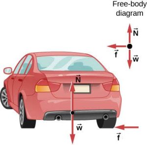
- (Figure) shows the forces acting on the car on an unbanked (level ground) curve. Friction is to the left, or toward the center of the turn, keeping the car from slipping, and is the only horizontal force acting on the car. We know that the maximum static friction (at which the tires roll but do not slip) is [latex]{\mu }_{\text{s}}N,[/latex] where [latex]{\mu }_{\text{s}}[/latex] is the static coefficient of friction and N is the normal force. The normal force, acting on the car, is equal to the car’s weight in this particular case, since
[latex]\sum {F_z} = ma_z[/latex]
[latex]N - w = m(0)[/latex]
[latex]N - mg = 0[/latex],
so [latex]N=mg.[/latex] Thus the static frictional force in this situation is
Now we also have a relationship between the frictional force and the linear speed of the car:
We solve this for [latex]{\mu }_{\text{s}},[/latex] noting that mass cancels, and obtain
Substituting the knowns,
(Because coefficients of friction are approximate, the answer is given to only two digits.)
Significance
The coefficient of friction found in part (b) is much smaller than is typically found between tires and roads. The car still negotiates the curve if the coefficient is greater than 0.13, because static friction is a responsive force, able to assume a value less than but no more than [latex]{\mu }_{\text{s}}N.[/latex] A higher coefficient would also allow the car to negotiate the curve at a higher speed, but if the coefficient of friction is less, the maximum safe speed would be less than 25 m/s. Note that the mass of the car cancels, implying that, in this example, it does not matter how heavily loaded the car is to negotiate the turn. Mass cancels because friction is proportional to the normal force, which in turn is proportional to mass. If the surface of the road were banked, the normal force would be less than the weight of the car, as discussed shortly.
Check Your Understanding 6.9
A car moving at 96.8 km/h travels around a circular curve of radius 182.9 m on a flat country road. What must be the minimum coefficient of static friction to keep the car from slipping?
In the example, notice that the static frictional force between the tires and the road, [latex]{\stackrel{\to }{f}}[/latex], is always perpendicular to the path and points to the center of curvature. Note that if you solve the expression obtained in the example using Newton's Second Law for r, you get
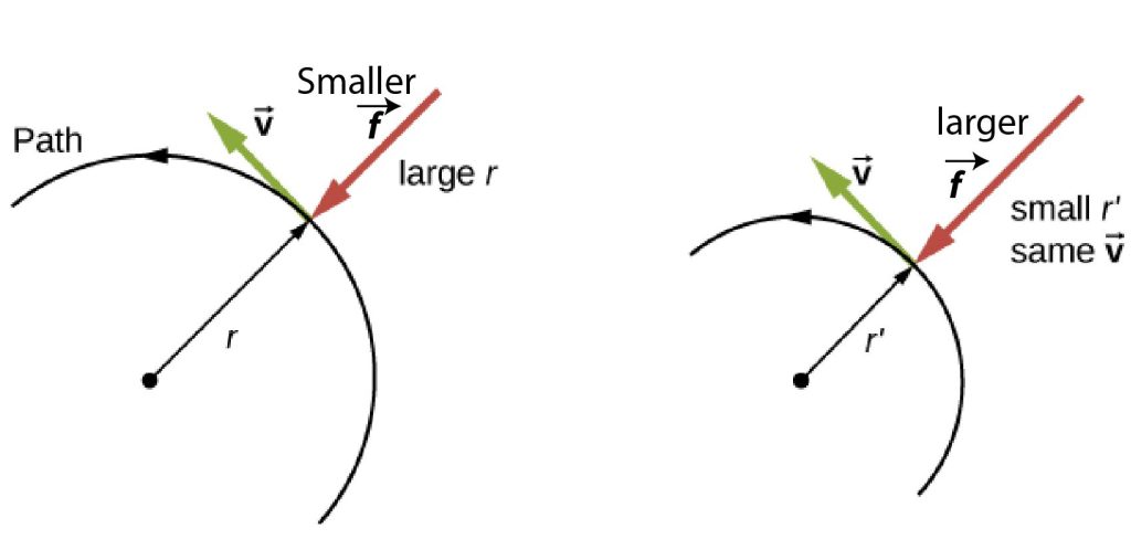
This implies that for a given mass and velocity, a large static frictional force causes a small radius of curvature—that is, a tight turn, as in (Figure). The larger the static frictional force, [latex]{f},[/latex] the smaller the radius of curvature r and the sharper the turn. The second curve has the same v, but a larger [latex]{f}[/latex] produces a smaller r′.
Banked Curves
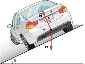
Let us now consider banked curves, where the slope of the road helps you negotiate the curve (Figure). The greater the angle [latex]\theta[/latex], the faster you can take the curve. Racetracks for bikes as well as cars, for example, often have steeply banked curves. In an “ideally banked curve,” the angle [latex]\theta[/latex] is such that you can negotiate the curve at a certain speed without the aid of friction between the tires and the road. We will derive an expression for the banking angle, [latex]\theta[/latex], for an ideally banked curve and consider an example related to it.
For ideal banking, the only forces acting on the car are the weight force exerted on the car by the earth and the normal force exerted on the car by the roadway, since we are ignoring any effects of friction in the ideal case.
(Figure) shows a free-body diagram for a car on a frictionless banked curve. If the angle [latex]\theta[/latex] is ideal for the speed and radius, then only two external forces act on the car: its weight [latex]\stackrel{\to }{w}[/latex] and the normal force of the road [latex]\stackrel{\to }{N}.[/latex] Only the normal force has a component along the radial direction (horizontal in this case). Keeping in mind that the radial component of the normal force is [latex]N_r = N \text{sin}\phantom{\rule{0.2em}{0ex}}\theta[/latex] and designating the [latex]+r[/latex] direction to point toward the center of the circular path around which the car travels:
[latex]\sum{F_r} = ma_r[/latex]
Because the car does not leave the surface of the road, the net vertical force must be zero. From (Figure), we see that the vertical component of the normal force is [latex]N_y = N\phantom{\rule{0.2em}{0ex}}\text{cos}\phantom{\rule{0.2em}{0ex}}\theta ,[/latex] and the only other vertical force is the car’s weight. These must be equal in magnitude; applying Newton's Second Law along the vertical axis:
[latex]\sum{F_y} = ma_y[/latex]
[latex]N \text{cos}\theta - w = m(0)[/latex]
Now we can combine these two equations to eliminate N and get an expression for [latex]\theta[/latex]. Solving the second equation for [latex]N,[/latex]:
[latex]N = \frac{mg}{\text{cos}\theta}[/latex]
Substituting this into the first yields
Taking the inverse tangent gives
This expression can be understood by considering how [latex]\theta[/latex] depends on v and r, though again only for ideal banking. A large [latex]\theta[/latex] is obtained for a large v and a small r. That is, roads must be steeply banked for high speeds and sharp curves. Friction helps, because it allows you to take the curve at a certain range of greater or lower speeds without skidding than if the curve were frictionless. Note that the banking angle, [latex]\theta,[/latex] does not depend on the mass of the vehicle.
You may notice that the FBD of the car in this case of a car traveling around a banked curve is the very same as the FBD of an object sliding on a ramp where friction between the object and ramp is negligible. As you go through this example, please note that we analyze this type of problem using horizontal and vertical axes rather than the tilted axis system used in solving problems with an object on an inclined plane. Why the difference in approaches? The difference in approaches occurs because of the direction of the acceleration of the object in question. As the car travels around the banked curve, it moves around a horizontal circle. The direction of the acceleration of the car is toward the center of the circular path since the car is assumed to travel around the curve with a constant speed. We choose one axis direction to align with the acceleration of the car (horizontal). In the case of the object sliding along an incline/ramp, the direction of the acceleration of the object was down the ramp. There, too, we chose one axis to align with the direction of the acceleration of the object (tilted; down the ramp). We typically use the direction of the acceleration to determine one axis of our system since all of the acceleration of the object is fully along this axis. We then use axes perpendicular to this first axis to complete our coordinate system, noting that there is no acceleration of the object along these other perpendicular axes.
What Is the Ideal Speed to Take a Steeply Banked Tight Curve?
Curves on some test tracks and race courses, such as Daytona International Speedway in Florida, are very steeply banked. This banking, with the aid of tire friction and very stable car configurations, allows the curves to be taken at very high speed. To illustrate, calculate the speed at which a 100.0-m radius curve banked at [latex]31.0\text{°}[/latex] should be driven if the road were frictionless.
Strategy
Because we derived the result starting from Newton's Laws above, we will use the expression for the ideal angle of a banked curve. On an exam, you should be able to solve any problem similar to those encountered in Chapters 5 and 6 of this text starting from Newton's Laws unless your instructor tells you otherwise. It is good practice to solve all homework problems starting from Newton's Laws rather than derived results. We note that all terms in the expression for the ideal angle of a banked curve except for speed are known; thus, we need only rearrange it so that speed appears on the left-hand side and then substitute known quantities.
Solution
Starting with
we get
Significance
This is just about 54 mph ([latex]\approx[/latex]87 km/h). Tire friction enables a vehicle to take the curve at significantly higher speeds, typical of those observed as cars race around the track at Daytona.
Airplanes also make turns by banking. The lift force, due to the force of the air on the wing, acts at right angles to the wing. When the airplane banks, the pilot is obtaining greater lift than necessary for level flight. The vertical component of lift balances the airplane’s weight, and the horizontal component accelerates the plane. The banking angle shown in (Figure) is given by [latex]\theta[/latex]. We analyze the forces in the same way we treat the case of the car rounding a banked curve.

Inertial Forces and Noninertial (Accelerated) Frames: The Coriolis Force
What do taking off in a jet airplane, turning a corner in a car, riding a merry-go-round, and the circular motion of a tropical cyclone have in common? Each exhibits inertial forces—forces that merely seem to arise from motion, because the observer’s frame of reference is accelerating or rotating. When taking off in a jet, most people would agree it feels as if you are being pushed back into the seat as the airplane accelerates down the runway. Yet a physicist would say that you tend to remain stationary while the seat pushes forward on you, consistent with Newton's First Law. An even more common experience occurs when you make a tight curve in your car—say, to the right (Figure). You feel as if you are thrown (that is, forced) toward the left relative to the car. Again, a physicist would say that this occurs not because you are experiencing a force from the left but rather you are going in a straight line (recall Newton’s first law) while the car moves to the right.
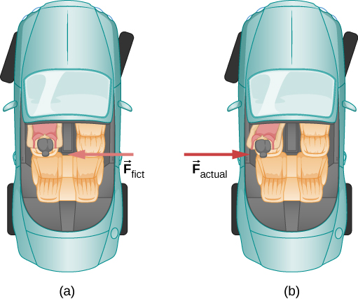
We can reconcile these points of view by examining the frames of reference used. Let us concentrate on people in a car. Passengers instinctively use the accelerating frame of reference of the car as a frame of reference, whereas a physicist might use Earth. The physicist might make this choice because Earth is nearly an inertial frame of reference, in which all forces have an identifiable physical origin. In such a frame of reference, Newton’s laws of motion take the form given in Newton’s Laws of Motion. The car is a noninertial frame of reference because it is an accelerated reference frame since its velocity is changing in time. The force to the left sensed by car passengers is an inertial force having no physical origin (it is due purely to the inertia of the passenger, not to some physical cause such as tension, friction, or gravitation). The car, as well as the driver, is actually accelerating to the right. This inertial force is said to be an inertial force, also called a fictitious force, because it does not have a physical origin, such as gravity.
A physicist will choose whatever reference frame is most convenient for the situation being analyzed. There is no problem to a physicist in including inertial forces and Newton’s second law, as usual, if that is more convenient, for example, on a merry-go-round or on a rotating planet. Noninertial (accelerated) frames of reference are used when it is useful to do so. Different frames of reference must be considered in discussing the motion of an astronaut in a spacecraft traveling at speeds near the speed of light, as you will appreciate in the study of the special theory of relativity.
Let us now take a mental ride on a merry-go-round—specifically, a rapidly rotating playground merry-go-round (Figure). You take the merry-go-round to be your frame of reference because you rotate together. When rotating in that noninertial frame of reference, you feel an inertial force that tends to throw you outward, away from the center of the circular path; this is often referred to as a centrifugal force. Centrifugal force is a commonly used term, but it does not actually exist. You must hang on tightly to counteract your inertia (which people often refer to as centrifugal force). In Earth’s frame of reference, there is no force trying to throw you off; we emphasize that centrifugal force is a fiction. You must hang on to make yourself go in a circle because otherwise you would go in a straight line, right off the merry-go-round, in keeping with Newton’s first law. But the force you exert acts toward the center of the circle.

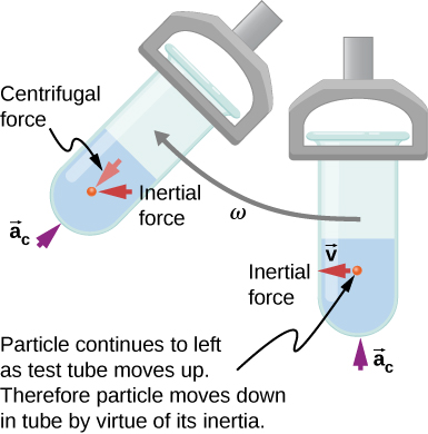
This inertial effect, carrying you away from the center of rotation, is put to good use in centrifuges (Figure). A centrifuge spins a sample very rapidly, as mentioned earlier in this chapter. Viewed from the rotating frame of reference, the inertial force throws particles outward, hastening their sedimentation. The greater the angular velocity, the greater the centrifugal force. But what really happens is that the inertia of the particles carries them along a line tangent to the circle while the test tube is forced in a circular path by the normal force exerted on the test tube by the surface of the centrifuge.
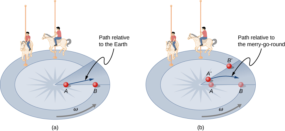
Let us now consider what happens if something moves in a rotating frame of reference. For example, what if you slide a ball directly away from the center of the merry-go-round, as shown in (Figure)? The ball follows a straight path relative to Earth (assuming negligible friction) and a path curved to the right on the merry-go-round’s surface. A person standing next to the merry-go-round sees the ball moving straight and the merry-go-round rotating underneath it. In the merry-go-round’s frame of reference, we explain the apparent curve to the right by using an inertial force, called the Coriolis force, which causes the ball to curve to the right. The Coriolis force can be used by anyone in that frame of reference to explain why objects follow curved paths and allows us to apply Newton’s laws in noninertial frames of reference.
Up until now, we have considered Earth to be an inertial frame of reference with little or no worry about effects due to its rotation. Yet such effects do exist—in the rotation of weather systems, for example. Most consequences of Earth’s rotation can be qualitatively understood by analogy with the merry-go-round. Viewed from above the North Pole, Earth rotates counterclockwise, as does the merry-go-round in (Figure). As on the merry-go-round, any motion in Earth’s Northern Hemisphere experiences a Coriolis force to the right. Just the opposite occurs in the Southern Hemisphere; there, the force is to the left. Because Earth’s angular velocity is small, the Coriolis force is usually negligible, but for large-scale motions, such as wind patterns, it has substantial effects.
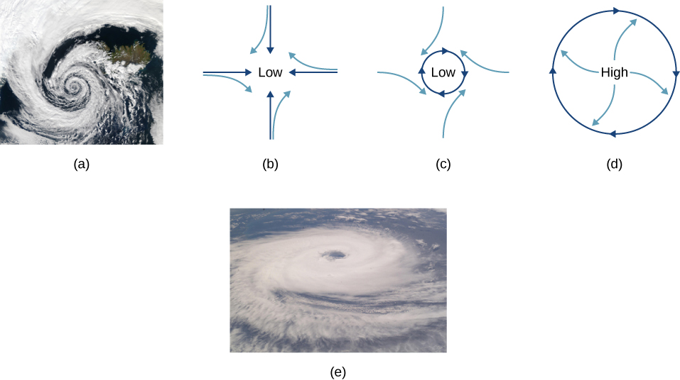
The Coriolis force causes hurricanes in the Northern Hemisphere to rotate in the counterclockwise direction, whereas tropical cyclones in the Southern Hemisphere rotate in the clockwise direction. (The terms hurricane, typhoon, and tropical storm are regionally specific names for cyclones, which are storm systems characterized by low pressure centers, strong winds, and heavy rains.) (Figure) helps show how these rotations take place. Air flows toward any region of low pressure, and tropical cyclones contain particularly low pressures. Thus winds flow toward the center of a tropical cyclone or a low-pressure weather system at the surface. In the Northern Hemisphere, these inward winds are deflected to the right, as shown in the figure, producing a counterclockwise circulation at the surface for low-pressure zones of any type. Low pressure at the surface is associated with rising air, which also produces cooling and cloud formation, making low-pressure patterns quite visible from space. Conversely, wind circulation around high-pressure zones is clockwise in the Southern Hemisphere but is less visible because high pressure is associated with sinking air, producing clear skies.
The rotation of tropical cyclones and the path of a ball on a merry-go-round can just as well be explained by inertia and the rotation of the system underneath. When noninertial frames are used, inertial forces, such as the Coriolis force, must be invented to explain the curved path. There is no identifiable physical source for these inertial forces. In an inertial frame, inertia explains the path, and no force is found to be without an identifiable source. Either view allows us to describe nature, but a view in an inertial frame is the simplest in the sense that all forces have origins and explanations.
Reading Check
