
10.8: Work and Power for Rotational Motion
Learning Objectives
By the end of this section, you will be able to:
- Use the work-energy theorem to analyze rotation to find the work done on a system when it is rotated about a fixed axis for a finite angular displacement
- Solve for the angular velocity of a rotating rigid body using the work-energy theorem
- Find the power delivered to a rotating rigid body given the applied torque and angular velocity
- Summarize the rotational variables and equations and relate them to their translational counterparts
Thus far in the chapter, we have extensively addressed kinematics and dynamics for rotating rigid bodies around a fixed axis. In this final section, we define work and power within the context of rotation about a fixed axis, which has applications to both physics and engineering. The discussion of work and power makes our treatment of rotational motion almost complete, with the exception of rolling motion and angular momentum, which are discussed in Angular Momentum. We begin this section with a treatment of the work-energy theorem for rotation.
Work for Rotational Motion
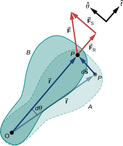
Now that we have determined how to calculate kinetic energy for rotating rigid bodies, we can proceed with a discussion of the work done on a rigid body rotating about a fixed axis. (Figure) shows a rigid body that has rotated through an angle [latex]d\theta[/latex] from A to B while under the influence of a force [latex]\stackrel{\to }{F}[/latex]. The external force [latex]\stackrel{\to }{F}[/latex] is applied to point P, whose position is [latex]\stackrel{\to }{r}[/latex], and the rigid body is constrained to rotate about a fixed axis that is perpendicular to the page and passes through O. The rotational axis is fixed, so the vector [latex]\stackrel{\to }{r}[/latex] moves in a circle of radius r, and the vector [latex]d\stackrel{\to }{s}[/latex] is perpendicular to [latex]\stackrel{\to }{r}.[/latex]
From (Figure), we have
Thus,
Note that [latex]d\stackrel{\to }{r}[/latex] is zero because [latex]\stackrel{\to }{r}[/latex] is fixed on the rigid body from the origin O to point P. Using the definition of work, we obtain
where we used the identity [latex]\stackrel{\to }{a}·\left(\stackrel{\to }{b}\phantom{\rule{0.2em}{0ex}}×\phantom{\rule{0.2em}{0ex}}\stackrel{\to }{c}\right)=\stackrel{\to }{b}·\left(\stackrel{\to }{c}\phantom{\rule{0.2em}{0ex}}×\phantom{\rule{0.2em}{0ex}}\stackrel{\to }{a}\right)[/latex]. Noting that [latex]\left(\stackrel{\to }{r}\phantom{\rule{0.2em}{0ex}}×\phantom{\rule{0.2em}{0ex}}\sum \stackrel{\to }{F}\right)=\sum \stackrel{\to }{\tau }[/latex], we arrive at the expression for the rotational work done on a rigid body:
The total work done on a rigid body is the sum of the torques integrated over the angle through which the body rotates. The incremental work is
where we have taken the dot product in (Figure), leaving only torques along the axis of rotation. In a rigid body, all particles rotate through the same angle; thus the work of every external force is equal to the torque times the common incremental angle [latex]d\theta[/latex]. The quantity [latex]\left(\sum _{i}{\tau }_{i}\right)[/latex] is the net torque on the body due to external forces.
Similarly, we found the kinetic energy of a rigid body rotating around a fixed axis by summing the kinetic energy of each particle that makes up the rigid body. Since the work-energy theorem [latex]{W}_{i}=\text{Δ}{K}_{i}[/latex] is valid for each particle, it is valid for the sum of the particles and the entire body.
The work-energy theorem for a rigid body rotating around a fixed axis is
where
and the rotational work done by a net force rotating a body from point A to point B is
We give a strategy for using this equation when analyzing rotational motion.
- Identify the forces on the body and draw a free-body diagram. Calculate the torque for each force.
- Calculate the work done during the body’s rotation by every torque.
- Apply the work-energy theorem by equating the net work done on the body to the change in rotational kinetic energy.
Let’s look at two examples and use the work-energy theorem to analyze rotational motion.
Rotational Work and Energy
A [latex]12.0\phantom{\rule{0.2em}{0ex}}\text{N}·\text{m}[/latex] torque is applied to a flywheel that rotates about a fixed axis and has a moment of inertia of [latex]30.0\phantom{\rule{0.2em}{0ex}}\text{kg}·{\text{m}}^{2}[/latex]. If the flywheel is initially at rest, what is its angular velocity after it has turned through eight revolutions?
Strategy
We apply the work-energy theorem. We know from the problem description what the torque is and the angular displacement of the flywheel. Then we can solve for the final angular velocity.
Solution
The flywheel turns through eight revolutions, which is [latex]16\pi[/latex] radians. The work done by the torque, which is constant and therefore can come outside the integral in (Figure), is
We apply the work-energy theorem:
With [latex]\tau =12.0\phantom{\rule{0.2em}{0ex}}\text{N}·\text{m},{\theta }_{B}-{\theta }_{A}=16.0\pi \phantom{\rule{0.2em}{0ex}}\text{rad},\phantom{\rule{0.2em}{0ex}}I=30.0\phantom{\rule{0.2em}{0ex}}\text{kg}·{\text{m}}^{2},\phantom{\rule{0.2em}{0ex}}\text{and}\phantom{\rule{0.2em}{0ex}}{\omega }_{A}=0[/latex], we have
Therefore,
This is the angular velocity of the flywheel after eight revolutions.
Significance
The work-energy theorem provides an efficient way to analyze rotational motion, connecting torque with rotational kinetic energy.
Rotational Work: A Pulley
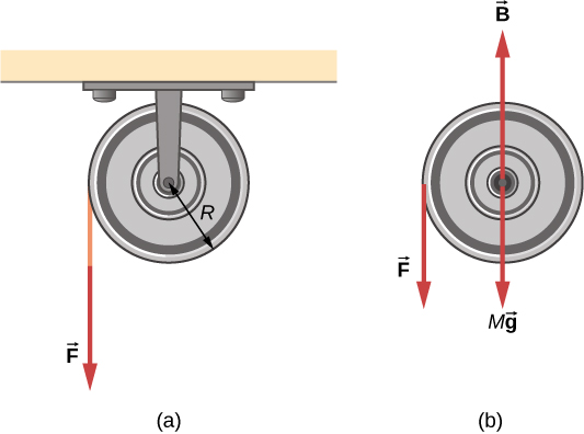
A string wrapped around the pulley in (Figure) is pulled with a constant downward force [latex]\stackrel{\to }{F}[/latex] of magnitude 50 N. The radius R and moment of inertia I of the pulley are 0.10 m and [latex]2.5\phantom{\rule{0.2em}{0ex}}×\phantom{\rule{0.2em}{0ex}}{10}^{-3}{\text{kg-m}}^{2}[/latex], respectively. If the string does not slip, what is the angular velocity of the pulley after 1.0 m of string has unwound? Assume the pulley starts from rest.
Strategy
Looking at the free-body diagram, we see that neither [latex]\stackrel{\to }{B}[/latex], the force on the bearings of the pulley, nor[latex]M\stackrel{\to }{g}[/latex], the weight of the pulley, exerts a torque around the rotational axis, and therefore does no work on the pulley. As the pulley rotates through an angle [latex]\theta ,[/latex] [latex]\stackrel{\to }{F}[/latex] acts through a distance d such that [latex]d=R\theta .[/latex]
Solution
Since the torque due to [latex]\stackrel{\to }{F}[/latex] has magnitude [latex]\tau =RF[/latex], we have
If the force on the string acts through a distance of 1.0 m, we have, from the work-energy theorem,
Solving for [latex]\omega[/latex], we obtain
Power for Rotational Motion
Power always comes up in the discussion of applications in engineering and physics. Power for rotational motion is equally as important as power in linear motion and can be derived in a similar way as in linear motion when the force is a constant. The linear power when the force is a constant is [latex]P=\stackrel{\to }{F}·\stackrel{\to }{v}[/latex]. If the net torque is constant over the angular displacement, (Figure) simplifies and the net torque can be taken out of the integral. In the following discussion, we assume the net torque is constant. We can apply the definition of power derived in Power to rotational motion. From Work and Kinetic Energy, the instantaneous power (or just power) is defined as the rate of doing work,
If we have a constant net torque, (Figure) becomes [latex]W=\tau \theta[/latex] and the power is
or
Torque on a Boat Propeller
A boat engine operating at [latex]9.0\phantom{\rule{0.2em}{0ex}}×\phantom{\rule{0.2em}{0ex}}{10}^{4}\phantom{\rule{0.2em}{0ex}}\text{W}[/latex] is running at 300 rev/min. What is the torque on the propeller shaft?
Strategy
We are given the rotation rate in rev/min and the power consumption, so we can easily calculate the torque.
Solution
Significance
It is important to note the radian is a dimensionless unit because its definition is the ratio of two lengths. It therefore does not appear in the solution.
Check Your Understanding 10.8
A constant torque of [latex]500\phantom{\rule{0.2em}{0ex}}\text{kN}·\text{m}[/latex] is applied to a wind turbine to keep it rotating at 6 rad/s. What is the power required to keep the turbine rotating?
Rotational and Translational Relationships Summarized
The rotational quantities and their linear analog are summarized in three tables. (Figure) summarizes the rotational variables for circular motion about a fixed axis with their linear analogs and the connecting equation, except for the centripetal acceleration, which stands by itself. (Figure) summarizes the rotational and translational kinematic equations. (Figure) summarizes the rotational dynamics equations with their linear analogs.
| Rotational | Translational | Relationship |
|---|---|---|
| [latex]\theta[/latex] | [latex]x[/latex] | [latex]\theta =\frac{s}{r}[/latex] |
| [latex]\omega[/latex] | [latex]{v}_{t}[/latex] | [latex]\omega =\frac{{v}_{t}}{r}[/latex] |
| [latex]\alpha[/latex] | [latex]{a}_{\text{t}}[/latex] | [latex]\alpha =\frac{{a}_{\text{t}}}{r}[/latex] |
| [latex]{a}_{\text{c}}[/latex] | [latex]{a}_{\text{c}}=\frac{{v}_{\text{t}}^{2}}{r}[/latex] |
| Rotational | Translational |
|---|---|
| [latex]{\theta }_{\text{f}}={\theta }_{0}+\stackrel{–}{\omega }t[/latex] | [latex]x={x}_{0}+\stackrel{–}{v}t[/latex] |
| [latex]{\omega }_{\text{f}}={\omega }_{0}+\alpha t[/latex] | [latex]{v}_{\text{f}}={v}_{0}+at[/latex] |
| [latex]{\theta }_{\text{f}}={\theta }_{0}+{\omega }_{0}t+\frac{1}{2}\alpha {t}^{2}[/latex] | [latex]{x}_{\text{f}}={x}_{0}+{v}_{0}t+\frac{1}{2}a{t}^{2}[/latex] |
| [latex]{\omega }_{\text{f}}^{2}={\omega }^{2}{}_{0}+2\alpha \left(\text{Δ}\theta \right)[/latex] | [latex]{v}_{\text{f}}^{2}={v}^{2}{}_{0}+2a\left(\text{Δ}x\right)[/latex] |
| Rotational | Translational |
|---|---|
| [latex]I=\sum _{i}{m}_{i}{r}_{i}^{2}[/latex] | m |
| [latex]K=\frac{1}{2}I{\omega }^{2}[/latex] | [latex]K=\frac{1}{2}m{v}^{2}[/latex] |
| [latex]\sum _{i}{\tau }_{i}=I\alpha[/latex] | [latex]\sum _{i}{\stackrel{\to }{F}}_{i}=m\stackrel{\to }{a}[/latex] |
| [latex]{W}_{AB}=\underset{{\theta }_{A}}{\overset{{\theta }_{B}}{\int }}\left(\sum _{i}{\tau }_{i}\right)d\theta[/latex] | [latex]W=\int \stackrel{\to }{F}·d\stackrel{\to }{s}[/latex] |
| [latex]P=\tau \omega[/latex] | [latex]P=\stackrel{\to }{F}·\stackrel{\to }{v}[/latex] |
