Chapter 4 Outline:

4.1 Population Size, Density, and Distribution

4.2 Demography, Age Structure, and Survivorship Curves

4.3 Exponential and Logistic Population Growth Models

4.4 Population Dynamics and Regulation

4.5 Demographic-Based Population Models – K-selected and r-selected Species

4.6 Case Study – Population Dynamics of Yellowstone Elk and Wolves

4.7 Case Study – Population Dynamics of the Wooly Mammoth – Why Did the Wooly Mammoth Go Extinct?

Learning Outcomes:

After studying this chapter, each student should be able to:

1. Describe how ecologists measure population size and density, and ways that populations may be distributed in nature
2. Explain the concept of demography, how age structure affects population growth, and what survivorship curves show
3. Differentiate between exponential and logistic growth, and the role of carrying capacity and intraspecific competition in limiting population growth
4. Describe various effects on Population Dynamics, such as density-dependent and density-independent environmental factors,
5. Differentiate between K-selected species and r-selected species
6. Describe the population dynamics of wolves and elk in the Yellowstone ecosystem, and changes in this ecosystem that occurred after wolf removal and after wolf reintroduction
7. Describe the possible roles that humans and climate change had in the decline and eventual extinction of the wooly mammoth

4.1 Population Size, Density, and Distribution

A population consists of all of the organisms of a particular species living within a specific area at the same time, which means that the organisms are likely interacting with each other in some way. The definition of a population can change with regards to location and the area being studied. For example, a scientist could study the population of saguaro cacti in Arizona, the United States, or in the entire Sonoran Desert.

Population size varies because of a number of factors. For example, births will add to a population, as will immigration of individuals into the area of the population in question. Deaths will decrease a population, as will immigration away from a population. Population size can be represented by an equation as follows:

Population Size = (Births Immigration) – (Deaths Emigration)

The study of any population usually begins by determining how many individuals of a particular species, or type, exist, and how closely associated they are with each other. Within a particular habitat, a population can be characterized by its population size (N), which is the total number of individuals present in a population, and its population density, which is the number of individuals within a specific area or volume. These characteristics, population size and population density, are the two main characteristics used to describe and understand populations.

For example, populations with more individuals may be more stable than smaller populations based on their genetic variability, which influences their potential to adapt to the environment. Alternatively, a member of a population with low population density (more spread out in the habitat), might have more difficulty finding a mate to reproduce compared to a population of higher density. As is shown in the graph in Figure 1, smaller organisms tend to be more densely distributed than larger organisms. Why do you think this is the case?

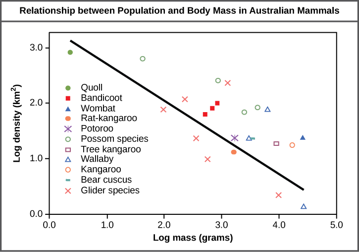
Figure 1. Australian mammals show a typical inverse relationship between population density and body size. (Credit: Relationship between Population and Body Mass in Australian Mammals, by OpenStax is licensed under CC-BY 4.0)

Population Research Methods

The most accurate way to determine population size is to simply count all of the individuals within the habitat. However, this method is often not logistically or economically feasible, especially when studying large habitats. Thus, scientists usually study populations by sampling a representative portion of each habitat and using this data to make inferences about the habitat as a whole.

A variety of methods can be used to sample populations to determine their size and density. For immobile organisms such as plants, or for very small and slow-moving organisms, a quadrat may be used (Figure 2). A quadrat is a way of marking off square areas within a habitat, either by staking out an area with sticks and string, or by the use of a wood, plastic, or metal square placed on the ground. After setting the quadrats, researchers then count the number of individuals that lie within their boundaries. Multiple quadrat samples are performed throughout the habitat at several random locations to estimate the population size and density within the entire habitat. The number and size of quadrat samples depends on the type of organisms under study and other factors, including the density of the organism. For example, if sampling daffodils, a 1 m² quadrat might be used. With giant redwoods, on the other hand, a larger quadrat of 100 m² might be employed. This ensures that enough individuals of the species are counted to get an accurate sample that correlates with the habitat, including areas not sampled.

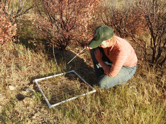
Figure 2. A scientist uses a quadrat to measure population size and density. (Credit: NPS Sonoran Desert Network)

For mobile organisms, such as mammals, birds, or fish, scientists use a technique called mark and recapture. This method involves marking a sample of captured animals in some way (such as tags, leg bands, paint, or other body markings), and then releasing them back into the environment to allow them to mix with the rest of the population. Later, researchers collect a new sample, including some individuals that are marked (recaptures) and some individuals that are unmarked (Figure 3).

Figure 3. Mark and recapture is used to measure the population size of mobile animals such as (a) bighorn sheep, (b) the California condor, and (c) salmon. (Credit a: modification of work by Neal Herbert, NPS; Credit b: modification of work by Pacific Southwest Region USFWS; Credit c: modification of work by Ingrid Taylar)

Using the ratio of marked and unmarked individuals, scientists determine how many individuals are in the sample. From this, calculations are used to estimate the total population size. This method assumes that the larger the population, the lower the percentage of tagged organisms that will be recaptured since they will have mixed with more untagged individuals. For example, if 80 deer are captured, tagged, and released into the forest, and later 100 deer are captured and 20 of them are already marked, we can estimate the population size (N) using the following equation:

N = M x S / R

 

Using our example, the deer population size would be:

  

There are some limitations to the mark and recapture method. Some animals from the first catch may learn to avoid capture in the second round, thus inflating population estimates. Alternatively, some animals may prefer to be trapped again (especially if a food reward is offered), resulting in an underestimate of population size. Also, some species may be harmed by the marking technique, reducing their survival. Scientists actually put a lot of thought into the design of tags to try and lessen the impact of a tag on an individual.

A variety of other techniques have been developed to study mobile organisms as well, including the electronic tracking of animals tagged with radio or satellite transmitters and the use of data from commercial fishing and trapping operations to estimate the size and health of populations and communities.

Species Distribution

In addition to measuring simple density, further information about a population can be obtained by looking at the distribution of the individuals. Species dispersion patterns (or distribution patterns) show the spatial relationship between members of a population within a habitat at a particular point in time. In other words, they show whether members of the species live close together or far apart, and what patterns are evident when they are spaced apart. Individuals in a population can be equally spaced apart, dispersed randomly with no predictable pattern, or clustered in groups. These are known as uniform, random, and clumped dispersion patterns, respectively (Figure 4).

Uniform dispersion is when organisms are equally spaced from one another. Uniform dispersion is observed in plants that secrete substances inhibiting the growth of nearby individuals (such as the release of toxic chemicals by the sage plant Salvia leucophylla or by creosote bushes Larrea tridentata). In animals uniform dispersion is often found in territorial animals like penguins, who peck at other penguins that come to close to their nest. Vicuñas, a llama-like animal, live in the high plains of Peru and maintain a defined territory around them, also resulting in uniform dispersion. 

Random dispersion is when organisms are not spaced in any particular pattern. They may be close together or far apart or anything in between. An example of random dispersion occurs with dandelions and other plants that have wind-dispersed seeds germinate wherever the seeds happen to fall in a favorable environment.

Clumped dispersion is noted when organisms are clustered together in groups. This type of dispersion may be seen in plants that drop their seeds straight to the ground, such as oak trees, or in animals that live in groups (schools of fish or herds of elk or elephants). Clumped dispersions may also be a function of habitat heterogeneity, meaning that resources in the habitat are not equally distributed, and the organisms are more likely to be found next to the resources.

Thus, the dispersion of the individuals within a population provides more information about how they interact with each other than does a simple density measurement. Just as lower density species might have more difficulty finding a mate, solitary species with a random distribution might have a similar difficulty when compared to social species clumped together in groups.

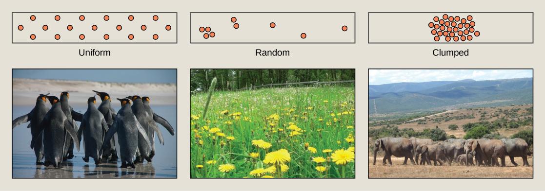
Figure 4. Species may have uniform, random, or clumped distribution. Territorial birds such as penguins tend to have uniform distribution. Plants such as dandelions with wind-dispersed seeds tend to be randomly distributed. Animals such as elephants that travel in groups exhibit clumped distribution. (Credit a: modification of work by Ben Tubby; Credit b: modification of work by Rosendahl; Credit c: modification of work by Rebecca Wood)

4.2 Demography, Age Structure, & Survivorship Curves

While population size and density describe a population at one particular point in time, scientists must use demography to study population dynamics. Demography is the statistical study of population changes over time, which includes studying birth rates, death rates, and life expectancies. Each of these measures, especially birth rates, may be affected by the population characteristics (size and density) described previously. For example, a large population size results in a higher birth rate because more potentially reproductive individuals are present. In contrast, a large population size can also result in a higher death rate because of competition for resources, the spread of disease between closely interacting individuals, and the accumulation of waste. Similarly, a higher population density or a clumped dispersion pattern results in more potential reproductive encounters between individuals, which can increase the birth rate. Lastly, a female-biased sex ratio (the ratio of females to males is high) or age structure (the proportion of population members at specific age ranges) composed of many individuals of reproductive age can also increase birth rates.

In addition, the demographic characteristics of a population can influence how the population grows or declines over time. If birth and death rates are equal, the population remains stable. However, the population size will increase if birth rates exceed death rates; the population will decrease if birth rates are less than death rates. Life expectancy is another important factor; the length of time individuals remain in the population impacts local resources, reproduction, and the overall health of the population. These demographic characteristics are often displayed in the form of a life table, or a graph of the population age structure, as shown in Figure 5.

 

   

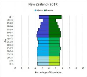
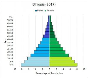
Figure 5. The graph on the left of New Zealand’s human age structure shows that this country has fairly stable human population growth, with equal numbers of individuals in the various age groups.  In contrast, the second graph shows that Ethiopia has a high rate of human population growth, with more young people than adults. Ethiopia’s human population size will increase rapidly in the future, based on the number of children who will pass through their reproductive stages in years to come. (Credit: Images courtesy of PopulationEducation)

The following TED talk shows how similar graphs are used to predict changes in populations:

 

Ted-Ed (2014, May 5) The Population Pyramid [Video – You Tube]. https://youtu.be/RLmKfXwWQtE

Survivorship Curves

Another tool used by population ecologists is a survivorship curve, which is a graph of the number of individuals surviving at each age interval plotted versus time (usually with data compiled from a life table). These curves allow us to compare the life histories of different populations (Figure 6). Note the graph below as the three major types of survivorship curves are described in the following paragraphs:

Humans and many large mammals exhibit a Type I survivorship curve because a high percentage of offspring survive their early and middle years. Death occurs predominantly in older individuals. These types of species usually have small numbers of offspring at one time, and they give a high amount of parental care to them to ensure their survival. Elephants and humans are good examples of this survivorship category.

Birds are an example of an intermediate or Type II survivorship curve because deaths occur at a regular rate throughout their life, with the likelihood of death at each age interval fairly uniform.  These organisms also may have relatively few offspring and provide significant parental care. 

Trees, alligators, marine invertebrates, and most fishes exhibit a Type III survivorship curve because very few of these organisms survive their younger years; however, those that make it to an old age are more likely to survive for a relatively long period of time. Organisms in this category usually have a very large number of offspring, but once they are born, little parental care is provided. Thus these offspring are “on their own” and vulnerable to predation, but their sheer numbers assure the survival of enough individuals to perpetuate the species.

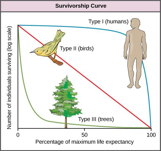
Figure 6. Survivorship curves show the distribution of individuals in a population according to age. (Credit: “Survivorship Curves” by OpenStax is licensed under CC-BY 4.0)

4.3 Exponential and Logistic Population Growth Models

Population ecologists make use of a variety of methods to model population dynamics. An accurate model should be able to describe the changes occurring in a population and predict future changes. Exponential growth models and logistic growth models are the two simplest models of population growth used to describe the rate of change in the size of a population over time. The first of these models, exponential growth, describes theoretical populations that increase in numbers without any limits to their growth.

The second model, logistic growth, introduces limits to reproductive growth that become more intense as the population size increases. Neither model adequately describes natural populations, but they provide points of comparison.

Exponential Growth

Exponential growth happens when an initial population increases by the same percentage over equal time increments or each generation, eventually resulting in very rapid growth.  Charles Darwin, in developing his theory of natural selection, was influenced by the exponential population growth described by the English clergyman Thomas Malthus. Malthus published a book in 1798 stating that populations with abundant natural resources grow very rapidly (exponentially); however, further growth may slow as resources are depleted. The early pattern of rapid, accelerating population growth is called exponential growth (Figure 7).

The rapid spread of Covid-19 in the human population is a stark example of exponential growth, and shows that J-shaped curve:

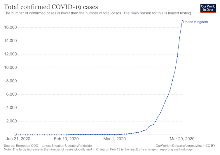
Figure 7. Exponential growth in the number of confirmed Covid-19 cases in the United Kingdom from January to March of 2020. (Source – European CDC)

Exponential growth can be easily observed in bacteria. Bacteria are prokaryotes and many types can reproduce approximately once per hour. If 1000 bacteria are placed in a large flask with an abundant supply of nutrients (so the nutrients will not become quickly depleted), the number of bacteria will have doubled from 1000 to 2000 after just an hour. In another hour, each of the 2000 bacteria will divide, producing 4000 bacteria. After the third hour, there should be 8000 bacteria in the flask. The important concept of exponential growth is that the growth rate—the number of organisms added in each reproductive generation—is itself increasing; that is, the population size is increasing at a greater and greater rate. After just one day (24 of these cycles), the population would have increased from 1000 to more than 16 billion bacteria. When the population size, N, is plotted over time, exponential growth shows a J-shaped growth curve  (Figure 8a).

The bacteria-in-a-flask example is not truly representative of the real world where resources are usually limited. However, when a species is introduced into a new habitat that it finds suitable, it may show exponential growth for a while. In the case of the bacteria in the flask, some bacteria will die during the experiment and thus not reproduce; therefore, the growth rate is lowered from a maximal rate in which there is no mortality. The growth rate of a population is largely determined by subtracting the death rate, D, (number organisms that die during an interval) from the birth rate, B, (number organisms that are born during an interval). If the birth rate is greater than the death rate, then the population is increasing in size. If the birth rate is less than the death rate, then the population is decreasing in size. If the birth rate and the death rate the same, then the size of the population is not changing.

Outside of the laboratory, however, where movement is not hindered, individuals may move out of the area of the population (emigration), thereby lowering the population size. Or, in contrast, individuals may move into the area defined by a population (immigration), thereby increasing the population. In the state of Arizona, bear populations in the mountains may dwindle if more food (such as ripening acorns) can be found at lower elevations, and bears emigrate to these new areas. The bear population gains numbers (by immigration) in these more food rich areas.

Logistic Growth

Logistic growth is different than exponential growth, because with logistic growth the population size does not continue to increase, because the critical resources available to the organisms are limited and run short.  Extended exponential growth is possible only when infinite natural resources are available; this is not the case in the real world. Charles Darwin recognized this fact in his description of the “struggle for existence,” which states that individuals will compete (with members of their own or other species) for limited resources. The successful ones are more likely to survive and pass on the traits that made them successful to the next generation (natural selection). To model population growth bearing in mind the reality of limited resources, population ecologists have developed the logistic growth model, as described below.

The Logistic Model

In the real world, with its limited resources, exponential growth cannot continue indefinitely. Exponential growth may occur in environments where there are few individuals and plentiful resources, but when the number of individuals gets large enough, resources will be depleted and the growth rate will slow down. Because of these limited resources, the growth rate will plateau or level off. Therefore, a graph of logistic growth yields a plot that looks like an “S”, or has an S-shaped curve (Figure 8b). This kind of growth is common in the real world, where resources are always limited,  slowing population growth. There are three different sections to an S-shaped curve. Initially, growth is exponential because there are few individuals and ample resources available. Then, as resources begin to become limited, the growth rate decreases. Finally, the growth rate levels off at the carrying capacity of the environment, with little change in population number over time.

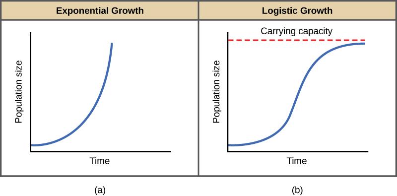
Figure 8. Graphs of (a) exponential growth, shown in a J-shaped curve and (b) logistic growth, shown in an S-shaped curve. (Credit: “Exponential and Logistic Growth Curves” by OpenStax is licensed under CC-BY 4.0)

Carrying Capacity

The size at which a population levels off, which is determined by the maximum population size that a particular environment can sustain, is called the carrying capacity, or K. In real populations, a growing population often overshoots its carrying capacity, and the death rate increases beyond the birth rate causing the population size to decline back to the carrying capacity or below it. Most populations usually fluctuate around the carrying capacity in an undulating fashion rather than existing right at it (Figure 9).

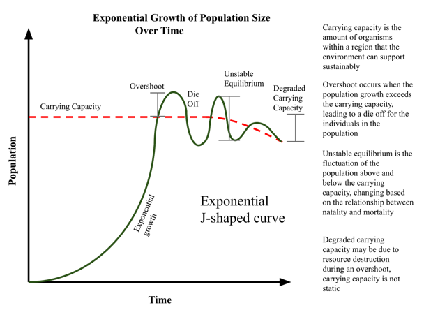
Figure 9. Graph showing population fluctuations around the carrying capacity. (Credit: Nchisick – own work, CC BY-SA 4.0, https://commons.wikimedia.org/w/index.php?curid=79117297)

Role of Intraspecific Competition

The logistic model assumes that every individual within a population will have equal access to resources and, thus, an equal chance for survival. For plants, the amount of water, sunlight, nutrients, and space to grow are the most important resources, whereas in animals, important resources include food, water, shelter, nesting space, and mates.

In the real world, variation among individuals within a population means that some individuals will be better adapted to their environment than others. The resulting competition for resources among population members of the same species is termed intraspecific competition. Intraspecific competition may not affect populations that are well below their carrying capacity, as resources are plentiful and all individuals can obtain what they need. However, as population size increases, this competition intensifies. In addition, the accumulation of waste products can reduce carrying capacity in an environment.

Examples of Logistic Growth

Yeast, a microscopic fungus used to make bread and alcoholic beverages, exhibits the classical S-shaped curve when grown in a test tube (Figure 10a). Its population growth levels off as the individuals in the population deplete the nutrients that are necessary for their growth and reproduction. In the real world, however, there are variations to this idealized curve. An example in a wild population is the population growth of harbor seals, which also levels off as the population uses all available resources (Figure 10b). In both examples, the population size exceeds the carrying capacity for short periods of time and then falls below the carrying capacity afterwards. This fluctuation in population size continues to occur as the population oscillates around its carrying capacity. Still, even with this oscillation, the logistic model is confirmed.

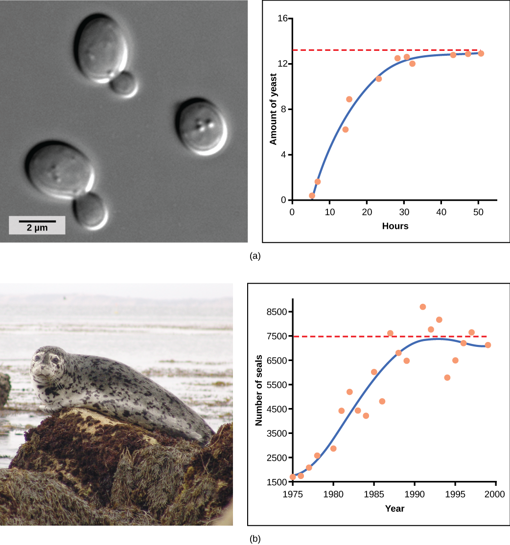
Figure 10. (a) Yeast grown in ideal conditions in a test tube shows a classical S-shaped logistic growth curve, whereas (b) a natural population of seals shows real-world fluctuation. (Credit: scale-bar data from Matt Russell)

4.4 Population Dynamics and Regulation

The logistic model of population growth, while valid in many natural populations and a useful model, is a simplification of real-world population dynamics. Implicit in the model is that the carrying capacity of the environment does not change, which is not the case. The carrying capacity varies annually. For example, some summers are hot and dry whereas others are cold and wet; in many areas, the carrying capacity during the winter is much lower than it is during the summer. Also, natural events such as earthquakes, volcanoes, and fires can alter an environment and hence its carrying capacity. Additionally, populations do not usually exist in isolation. They share the environment with other species, competing with them for the same resources (interspecific competition). These factors are also important to understanding how a specific population will grow.

Population growth is regulated in a variety of ways. These are grouped into density-dependent factors, in which the density of the population affects growth rate and mortality, and density-independent factors, which cause mortality in a population regardless of population density. Wildlife biologists, in particular, want to understand both types because this helps them manage populations to prevent extinction or overpopulation.

Density-dependent Regulation

Most density-dependent factors are biological in nature and include predation, interspecific and intraspecific competition, and parasites. Usually, the denser a population is, the greater its mortality rate. In addition, low prey density increases the mortality of its predator because it has more difficulty locating its food source. Also, when the population is denser, diseases spread more rapidly among the members of the population, which increases the mortality rate.

Density dependent regulation was studied in a natural experiment with wild donkey populations on two sites in Australia.₂ On one site the population was reduced by a population control program; the population on the other site received no interference. The high-density plot was twice as dense as the low-density plot at the start of the experiment. From 1986 to 1987 the high-density plot saw no change in donkey density, while the low-density plot saw an increase in donkey density. The difference in the growth rates of the two populations was caused by a difference in mortality rates; not by a difference in birth rates. The number of offspring birthed by each mother was about the same in both populations and was therefore unaffected by density, but juveniles born in the denser population had a greater mortality rate caused by the mother’s malnutrition due to scarce high-quality food. Figure 11 shows the difference in age-specific mortalities in the two populations.

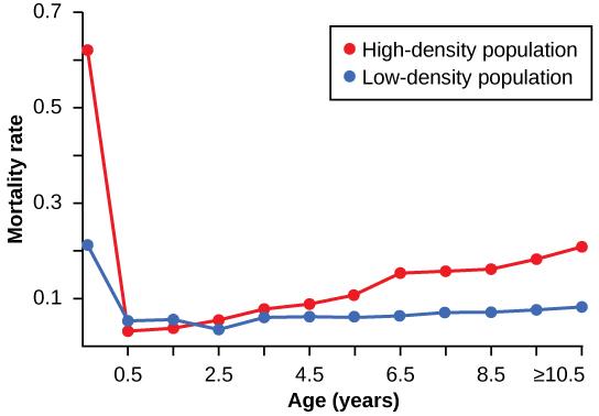
Figure 11. This graph shows the age-specific mortality rates for wild donkeys from high- and low-density populations. The juvenile mortality is much higher in the high-density population because of maternal malnutrition caused by a shortage of high-quality food. (Credit: “Age Specific Mortality Rates for Wild Donkeys” by OpenStax is licensed under CC-BY 4.0)

Density-independent and Density-dependent Factor Interactions

Density-independent regulation factors are typically physical in nature, causing mortality in a population regardless of its density. These factors include weather, natural disasters, and pollution. An individual deer will be killed in a forest fire regardless of how many deer happen to be in that area. Its chances of survival are the same whether the population density is high or low. The same holds true for cold winter weather.

In real-life situations, population regulation is very complicated and density-dependent and independent factors can interact. A dense population that suffers mortality from a density-independent cause will be able to recover differently than a sparse population. For example, a population of deer affected by a harsh winter will recover faster if there are more deer remaining to reproduce.

4.5 Demographic-Based Population Models – K-selected and r-selected Species

Population ecologists have hypothesized that suites, or groups, of characteristics may evolve in species that lead to particular adaptations to their environments. These adaptations impact the kind of population growth their species experience. Life history characteristics such as birth rates, age at first reproduction, the numbers of offspring, and even death rates evolve just like anatomy or behavior, leading to adaptations that affect population growth. Population ecologists have described a continuum of life-history “strategies” with K-selected species on one end and r-selected species on the other (figure 11) .

K-selected species are adapted to stable, predictable environments. Populations of K-selected species tend to exist close to their carrying capacity. These species tend to have larger, but fewer, offspring and contribute large amounts of resources to each offspring. Elephants and other large mammals would be examples of K-selected species.

r-selected species are adapted to unstable and unpredictable environments. They tend to have large numbers of small offspring but do not care for them. Animals that are r-selected do not provide a lot of resources or parental care to offspring, and the offspring are relatively self-sufficient at birth. Examples of r-selected species are marine invertebrates such as jellyfish and plants such as the dandelion (Figure 12).

 

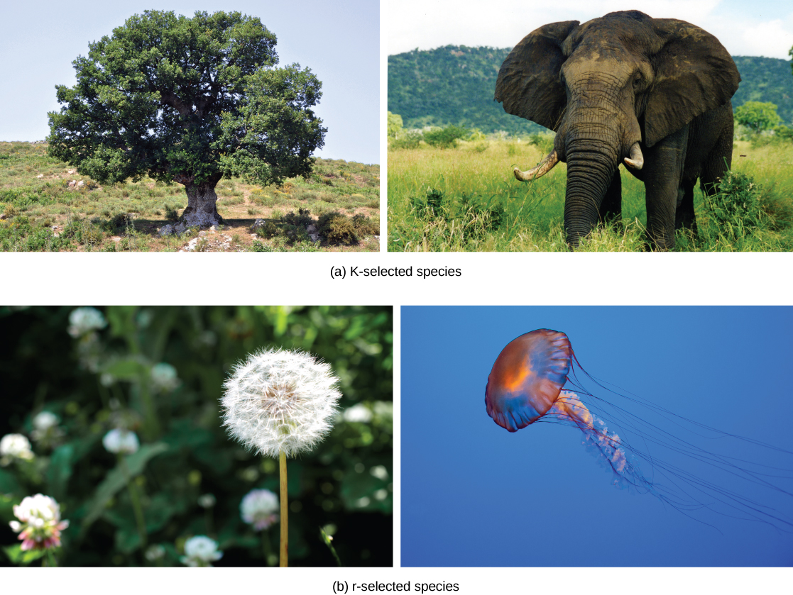
Figure 12. Examples of (a) K-selected and (b) r-selected species. (Credit: Creative Commons Attribution 4.0 International License)

The two extreme strategies are at two ends of a continuum on which real species life histories will exist. In addition, life history strategies do not need to evolve as suites, but can evolve independently of each other, so each species may have some characteristics that trend toward one extreme or the other. Table 1 shows many of the defining characteristics of r-selected and K-selected species.

Characteristic	r-selected	K-selected
Number of offspring	high	low
Parental care	low	high
Reproductive Maturity	early	late
Size of offspring	small	large
Independence at birth	early	late
Ability to learn	low	high
Lifespan	short	long
Early mortality	high	low

Table 1. This table shows the major characteristics of r- and K- selected species. Note that these are extremes and many species may fall between r- and K- descriptions. (Credit: Table created by Paul Bosch)

4.6 Case Study – Population Dynamics of Yellowstone Elk and Wolves

Wolves were an integral part of the ecosystem across much of the United States before European settlement (Figure 13). But as settlers moved west in the 1800s, they hunted native prey species such as pronghorn, deer, elk, and bison, and largely replaced this wildlife with domestic animals such as cattle and sheep. Suddenly lacking natural prey, wolves and other large carnivores began to attack domestic stock. Government sponsored programs tried to eliminate these carnivores with every tool at hand, such as hunting, trapping, and even large-scale poisoning of all carnivores. These programs greatly reduced and even eliminated large predators from much of the west.

In 1872 Yellowstone National Park was established to protect the natural habitat within its borders. But even in the park, wolves were considered detrimental to the herbivores in the park and were actively sought out and killed year after year. Between 1914 and 1926, for example, at least 135 wolves were killed within the park boundaries. At the time biologists did not understand the interconnected nature of ecosystems, with predator and prey in a balance that helped maintain both populations in a healthy state.

By the 1950s, wolves had been virtually eliminated from the continental United States, including within national parks. In Yellowstone, herbivores such as deer, elk, and bison increased in numbers to the point where they were damaging the very ecosystem that they depended on. There were so many elk, they ate all new growth along the rivers and even stripped larger trees of their bark during periods of extreme hunger, especially in the winter. With fewer trees to anchor soil near the rivers and streams, erosion increased dramatically. Smaller predators such as coyotes thrived in the absence of wolves, and decreased the population of smaller mammals, including rodents that birds of prey like golden eagles depended on.

In 1991, Congress provided funds to study how wolves might be reintroduced successfully to the Yellowstone ecosystem. By 1995, wolves that had been captured in Canada were habituated in large enclosures within Yellowstone National Park, fitted with radio collars, and then released into the wild. To increase genetic diversity, other wolves captured from different parts of Canada were released later that year and in 1996. Although some of these wolves moved out of the park and preyed on livestock, most found plenty of prey within the park. Funds were available to compensate ranchers outside of the park for any loss of livestock to wolves.

The healing of the ecosystem began quickly as the wolves began to prey on the large elk population in particular. Some elk were directly killed and eaten, lowering their population, but another important effect was not as predictable: the elk spent less and less time along the river banks, where they were most vulnerable to attack. The willows and other river bank (riparian) plants began to recover and areas that had not had new tree growth for decades began to grow into new forests. The problem of erosion began to decrease, and diverse species of wildlife started to return to the riparian areas. Beavers came back, with the trees again available as a food source, and their dams created small ponds, which attracted otters and other water related species. The Yellowstone ecosystem was recovering beyond expectations!

Some scientists had been concerned that the reintroduction of the wolves would have a negative impact on another endangered Yellowstone carnivore, the grizzly bear, as the bears and wolves competed for the same prey species. But wolves had just the opposite effect – the reduction in the elk population allowed berry and nut producing plants to flourish, important food sources for the bears. The grizzlies were also observed to drive the smaller wolves off their kills to eat the carrion themselves, also increasing available food for the bears.

What became clear from this history is that when populations of prey species are not kept in check by predators such as wolves, the prey species multiply beyond the carrying capacity of their ecosystem. In the case of Yellowstone, the elk herds grew to the point where they were eating young trees and shrubs down to the ground, which meant that their food supply was compromised and large numbers of animals starved to death, especially during the long Wyoming winters. The wolves themselves continue to multiply, but their numbers are expected to be kept in check by the availability of prey and competition with other large predators such as bears and mountain lions. Today biologists agree that the Yellowstone ecosystem is much healthier, with greater biodiversity, than before the reintroduction of wolves in the 1990s.

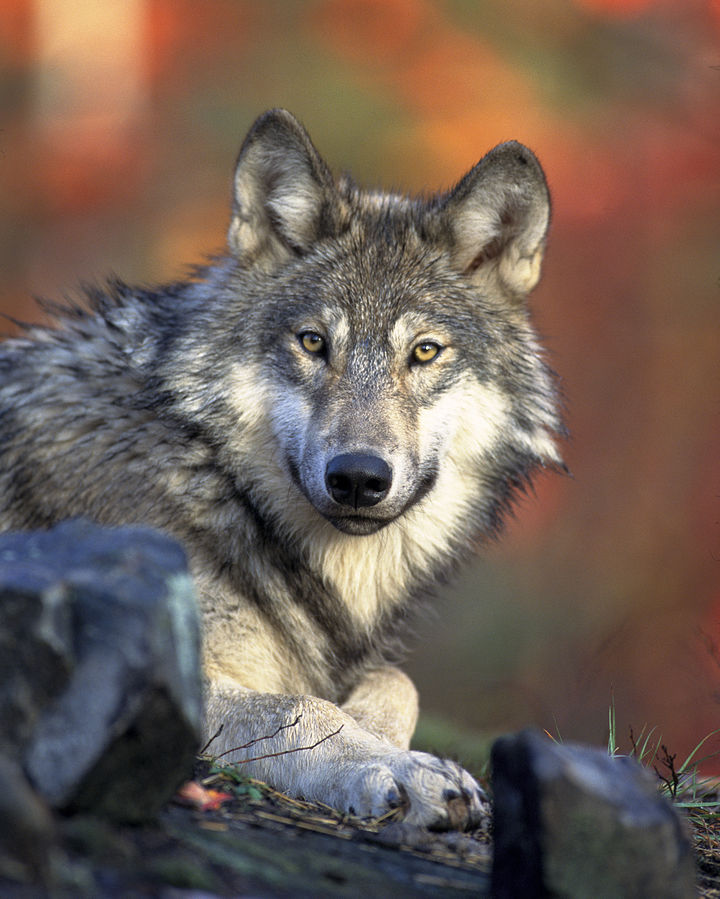
Figure 13. The gray wolf (Canis lupus) of the American West. (Credit: Gary Kramer, Public Domain)

View the following video to better understand the changes brought about by the reintroduction of the gray wolf to the Yellowstone National Park ecosystem. Note that the British narrator describes what we refer to as elk as “red deer”:

 

Sustainable Human (2014, Feb 13). How wolves change rivers. [Video – YouTube] https://youtu.be/ysa5OBhXz-Q

 

4.7 Case Study – Population Dynamics of the Wooly Mammoth – Why Did the Wooly Mammoth Go Extinct?

Woolly mammoths began to go extinct about 10,000 years ago, soon after paleontologists believe humans able to hunt them began to colonize North America and northern Eurasia (Figure 14). A mammoth population survived on Wrangel Island, in the East Siberian Sea, and was isolated from human contact until as recently as 1700 BC. We know a lot about these animals from carcasses found frozen in the ice of Siberia and other northern regions.

It is commonly thought that a combination of climate change and human hunting led to their extinction. A 2008 study estimated that climate change reduced the mammoth’s range from 3,000,000 square miles 42,000 years ago to 310,000 square miles 6,000 years ago. In addition to climate change and reduction of habitat, scientists demonstrated another important factor in the mammoth’s extinction – migration of human hunters across the Bering Strait to North America during the last ice age 20,000 years ago. Through archaeological evidence of kill sites, it is well documented that humans hunted these animals.

The maintenance of stable populations was and is very complex, with many interacting factors determining the outcome. It is important to remember that humans have always had an outsized effect on the population of other species. Many years ago, humans may have contributed to a species’ decline and extinction using little more than primitive hunting tools.

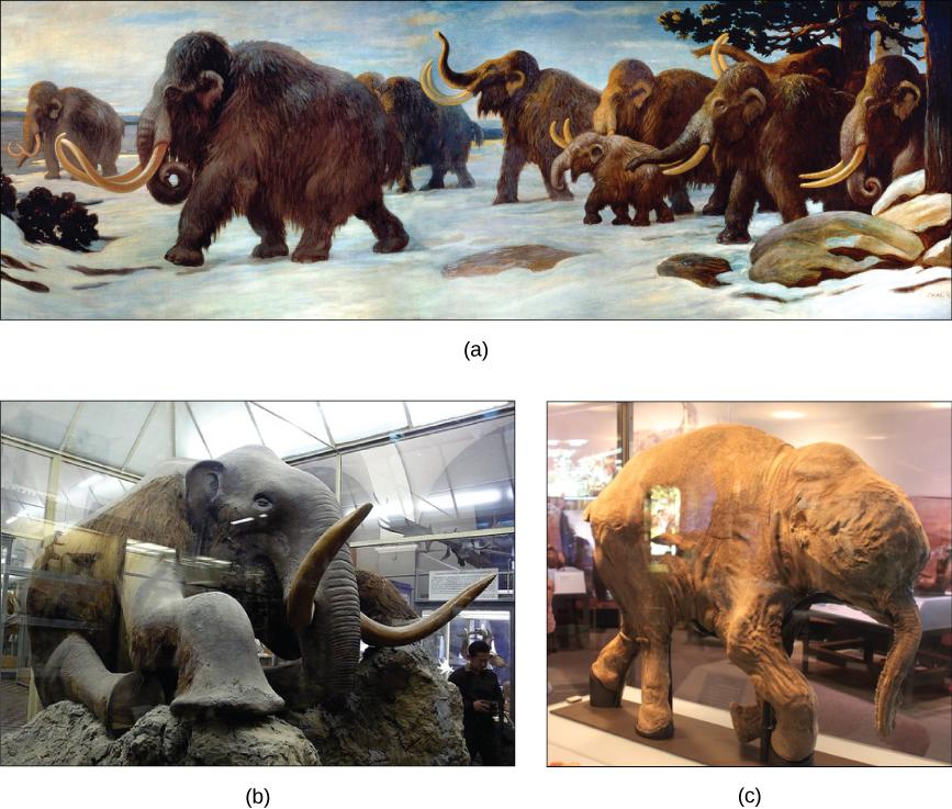
Figure 14. The three images include: (a) 1916 mural of a mammoth herd from the American Museum of Natural History, (b) the only stuffed mammoth in the world is in the Museum of Zoology located in St. Petersburg, Russia, and (c) a one-month-old baby mammoth, named Lyuba, discovered in Siberia in 2007. (Credit a: modification of work by Charles R. Knight; Credit b: modification of work by “Tanapon”/Flickr; Credit C: modification of work by Matt Howry)

The Natural History Museum in London created the following video, which addresses the extinction of the wooly mammoth, and provides further insight into what may have caused the loss of this species:

 

Natural History Museum, London England (2021, Nov 30). The last of the mammoths. [Video – YouTube] https://youtu.be/a2744xoqRKo?list=TLGGJ_334lo8hV4yNjA5MjAyMw

Attribution:

Content in this chapter includes original work created by Lauren Roberts and Paul Bosch as well as from the following sources, with some modifications:

Biology by OpenStax is licensed under CC BY 3.0.

Essentials of Environmental Science by Kamala Doršner is licensed under CC BY 4.0