
10 Chapter 10: Hypothesis Testing with Z
Setting up the hypotheses
When setting up the hypotheses with z, the parameter is associated with a sample mean (in the previous chapter examples the parameters for the null used 0). Using z is an occasion in which the null hypothesis is a value other than 0. For example, if we are working with mothers in the U.S. whose children are at risk of low birth weight, we can use 7.47 pounds, the average birth weight in the US, as our null value and test for differences against that. For now, we will focus on testing a value of a single mean against what we expect from the population.
Using birthweight as an example, our null hypothesis takes the form: H0: μ = 7.47 Notice that we are testing the value for μ, the population parameter, NOT the sample statistic ̅X (or M). We are referring to the data right now in raw form (we have not standardized it using z yet). Again, using inferential statistics, we are interested in understanding the population, drawing from our sample observations. For the research question, we have a mean value from the sample to use, we have specific data is – it is observed and used as a comparison for a set point.
As mentioned earlier, the alternative hypothesis is simply the reverse of the null hypothesis, and there are three options, depending on where we expect the difference to lie. We will set the criteria for rejecting the null hypothesis based on the directionality (greater than, less than, or not equal to) of the alternative.
If we expect our obtained sample mean to be above or below the null hypothesis value (knowing which direction), we set a directional hypothesis. Our alternative hypothesis takes the form based on the research question itself. In our example with birthweight, this could be presented as HA: μ > 7.47 or HA: μ < 7.47.
Note that we should only use a directional hypothesis if we have a good reason, based on prior observations or research, to suspect a particular direction. When we do not know the direction, such as when we are entering a new area of research, we use a non-directional alternative hypothesis. In our birthweight example, this could be set as HA: μ ≠ 7.47
In working with data for this course we will need to set a critical value of the test statistic for alpha (α) for use of test statistic tables in the back of the book. This is determining the critical rejection region that has a set critical value based on α.
Determining Critical Value from α
We set alpha (α) before collecting data in order to determine whether or not we should reject the null hypothesis. We set this value beforehand to avoid biasing ourselves by viewing our results and then determining what criteria we should use.
When a research hypothesis predicts an effect but does not predict a direction for the effect, it is called a non-directional hypothesis. To test the significance of a non-directional hypothesis, we have to consider the possibility that the sample could be extreme at either tail of the comparison distribution. We call this a two-tailed test.
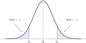
Figure 1. showing a 2-tail test for non-directional hypothesis for z for area C is the critical rejection region.
When a research hypothesis predicts a direction for the effect, it is called a directional hypothesis. To test the significance of a directional hypothesis, we have to consider the possibility that the sample could be extreme at one-tail of the comparison distribution. We call this a one-tailed test.
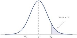
Figure 2. showing a 1-tail test for a directional hypothesis (predicting an increase) for z for area C is the critical rejection region.
Determining Cutoff Scores with Two-Tailed Tests
Typically we specify an α level before analyzing the data. If the data analysis results in a probability value below the α level, then the null hypothesis is rejected; if it is not, then the null hypothesis is not rejected. In other words, if our data produce values that meet or exceed this threshold, then we have sufficient evidence to reject the null hypothesis; if not, we fail to reject the null (we never “accept” the null). According to this perspective, if a result is significant, then it does not matter how significant it is. Moreover, if it is not significant, then it does not matter how close to being significant it is. Therefore, if the 0.05 level is being used, then probability values of 0.049 and 0.001 are treated identically. Similarly, probability values of 0.06 and 0.34 are treated identically. Note we will discuss ways to address effect size (which is related to this challenge of NHST).
When setting the probability value, there is a special complication in a two-tailed test. We have to divide the significance percentage between the two tails. For example, with a 5% significance level, we reject the null hypothesis only if the sample is so extreme that it is in either the top 2.5% or the bottom 2.5% of the comparison distribution. This keeps the overall level of significance at a total of 5%. A one-tailed test does have such an extreme value but with a one-tailed test only one side of the distribution is considered.
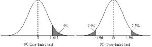
Figure 3. Critical value differences in one and two-tail tests. Photo Credit
Let’s review the set critical values for Z.
We discussed z-scores and probability in chapter 8. If we revisit the z-score for 5% and 1%, we can identify the critical regions for the critical rejection areas from the unit standard normal table.
- A two-tailed test at the 5% level has a critical boundary Z score of +1.96 and -1.96
- A one-tailed test at the 5% level has a critical boundary Z score of +1.64 or -1.64
- A two-tailed test at the 1% level has a critical boundary Z score of +2.58 and -2.58
- A one-tailed test at the 1% level has a critical boundary Z score of +2.33 or -2.33.
Review: Critical values, p-values, and significance level
There are two criteria we use to assess whether our data meet the thresholds established by our chosen significance level, and they both have to do with our discussions of probability and distributions. Recall that probability refers to the likelihood of an event, given some situation or set of conditions. In hypothesis testing, that situation is the assumption that the null hypothesis value is the correct value, or that there is no effect. The value laid out in H0 is our condition under which we interpret our results. To reject this assumption, and thereby reject the null hypothesis, we need results that would be very unlikely if the null was true.
Now recall that values of z which fall in the tails of the standard normal distribution represent unlikely values. That is, the proportion of the area under the curve as or more extreme than z is very small as we get into the tails of the distribution. Our significance level corresponds to the area under the tail that is exactly equal to α: if we use our normal criterion of α = .05, then 5% of the area under the curve becomes what we call the rejection region (also called the critical region) of the distribution. This is illustrated in Figure 4.
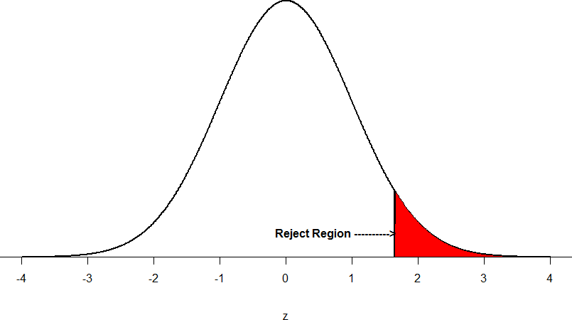
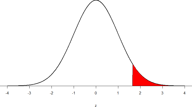
Figure 4: The rejection region for a one-tailed test
The shaded rejection region takes us 5% of the area under the curve. Any result which falls in that region is sufficient evidence to reject the null hypothesis.
The rejection region is bounded by a specific z-value, as is any area under the curve. In hypothesis testing, the value corresponding to a specific rejection region is called the critical value, zcrit (“z-crit”) or z* (hence the other name “critical region”). Finding the critical value works exactly the same as finding the z-score corresponding to any area under the curve like we did in Unit 1. If we go to the normal table, we will find that the z-score corresponding to 5% of the area under the curve is equal to 1.645 (z = 1.64 corresponds to 0.0405 and z = 1.65 corresponds to 0.0495, so .05 is exactly in between them) if we go to the right and -1.645 if we go to the left. The direction must be determined by your alternative hypothesis, and drawing then shading the distribution is helpful for keeping directionality straight.
Suppose, however, that we want to do a non-directional test. We need to put the critical region in both tails, but we don’t want to increase the overall size of the rejection region (for reasons we will see later). To do this, we simply split it in half so that an equal proportion of the area under the curve falls in each tail’s rejection region. For α = .05, this means 2.5% of the area is in each tail, which, based on the z-table, corresponds to critical values of z* = ±1.96. This is shown in Figure 5.
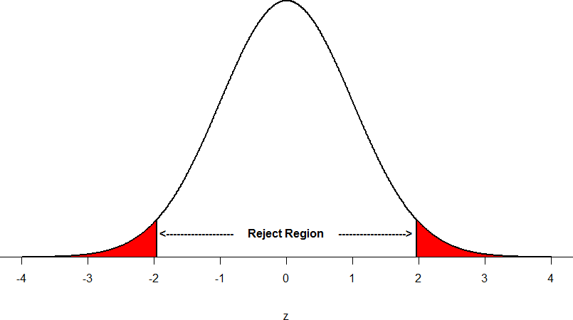
Figure 5: Two-tailed rejection region
Thus, any z-score falling outside ±1.96 (greater than 1.96 in absolute value) falls in the rejection region. When we use z-scores in this way, the obtained value of z (sometimes called z-obtained) is something known as a test statistic, which is simply an inferential statistic used to test a null hypothesis.
Calculate the test statistic: Z
Now that we understand setting up the hypothesis and determining the outcome, let’s examine hypothesis testing with z! The next step is to carry out the study and get the actual results for our sample. Central to hypothesis test is comparison of the population and sample means. To make our calculation and determine where the sample is in the hypothesized distribution we calculate the Z for the sample data.
Make a decision
To decide whether to reject the null hypothesis, we compare our sample’s Z score to the Z score that marks our critical boundary. If our sample Z score falls inside the rejection region of the comparison distribution (is greater than the z-score critical boundary) we reject the null hypothesis.
The formula for our z- statistic has not changed:
 where
where 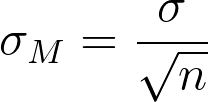
To formally test our hypothesis, we compare our obtained z-statistic to our critical z-value. If zobt > zcrit, that means it falls in the rejection region (to see why, draw a line for z = 2.5 on Figure 1 or Figure 2) and so we reject H0. If zobt < zcrit, we fail to reject. Remember that as z gets larger, the corresponding area under the curve beyond z gets smaller. Thus, the proportion, or p-value, will be smaller than the area for α, and if the area is smaller, the probability gets smaller. Specifically, the probability of obtaining that result, or a more extreme result, under the condition that the null hypothesis is true gets smaller.
Conversely, if we fail to reject, we know that the proportion will be larger than α because the z-statistic will not be as far into the tail. This is illustrated for a one- tailed test in Figure 6.
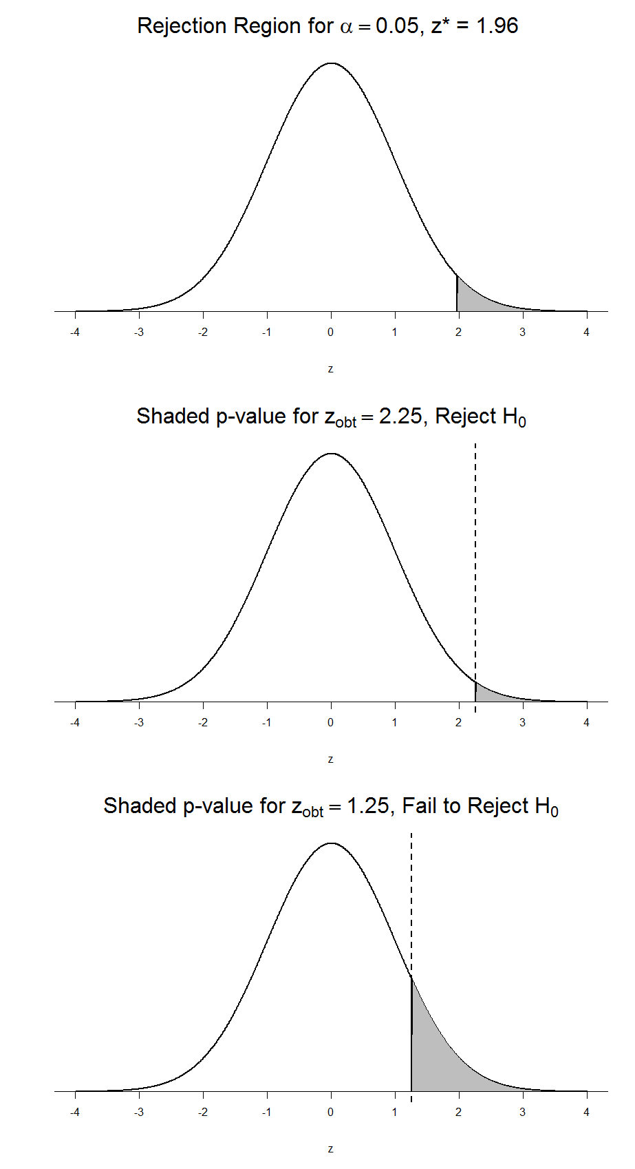
Figure 6. Relation between α, zobt, and p
When the null hypothesis is rejected, the effect is said to be statistically significant. Do not confuse statistical significance with practical significance. A small effect can be highly significant if the sample size is large enough.
Why does the word “significant” in the phrase “statistically significant” mean something so different from other uses of the word? Interestingly, this is because the meaning of “significant” in everyday language has changed. It turns out that when the procedures for hypothesis testing were developed, something was “significant” if it signified something. Thus, finding that an effect is statistically significant signifies that the effect is real and not due to chance. Over the years, the meaning of “significant” changed, leading to the potential misinterpretation.
Review: Steps of the Hypothesis Testing Process
The process of testing hypotheses follows a simple four-step procedure. This process will be what we use for the remained of the textbook and course, and though the hypothesis and statistics we use will change, this process will not.
Step 1: State the Hypotheses
Your hypotheses are the first thing you need to lay out. Otherwise, there is nothing to test! You have to state the null hypothesis (which is what we test) and the alternative hypothesis (which is what we expect). These should be stated mathematically as they were presented above AND in words, explaining in normal English what each one means in terms of the research question.
Step 2: Find the Critical Values
Next, we formally lay out the criteria we will use to test our hypotheses. There are two pieces of information that inform our critical values: α, which determines how much of the area under the curve composes our rejection region, and the directionality of the test, which determines where the region will be.
Step 3: Compute the Test Statistic
Once we have our hypotheses and the standards we use to test them, we can collect data and calculate our test statistic, in this case z. This step is where the vast majority of differences in future chapters will arise: different tests used for different data are calculated in different ways, but the way we use and interpret them remains the same.
Step 4: Make the Decision
Finally, once we have our obtained test statistic, we can compare it to our critical value and decide whether we should reject or fail to reject the null hypothesis. When we do this, we must interpret the decision in relation to our research question, stating what we concluded, what we based our conclusion on, and the specific statistics we obtained.
Example: Movie Popcorn
Let’s see how hypothesis testing works in action by working through an example. Say that a movie theater owner likes to keep a very close eye on how much popcorn goes into each bag sold, so he knows that the average bag has 8 cups of popcorn and that this varies a little bit, about half a cup. That is, the known population mean is μ = 8.00 and the known population standard deviation is σ =0.50. The owner wants to make sure that the newest employee is filling bags correctly, so over the course of a week he randomly assesses 25 bags filled by the employee to test for a difference (n = 25). He doesn’t want bags overfilled or under filled, so he looks for differences in both directions. This scenario has all of the information we need to begin our hypothesis testing procedure.
Step 1: State the Hypotheses
Our manager is looking for a difference in the mean cups of popcorn bags compared to the population mean of 8. We will need both a null and an alternative hypothesis written both mathematically and in words. We’ll always start with the null hypothesis:
H0: There is no difference in the cups of popcorn bags from this employee H0: μ = 8.00
Notice that we phrase the hypothesis in terms of the population parameter μ, which in this case would be the true average cups of bags filled by the new employee.
Our assumption of no difference, the null hypothesis, is that this mean is exactly
the same as the known population mean value we want it to match, 8.00. Now let’s do the alternative:
HA: There is a difference in the cups of popcorn bags from this employee HA: μ ≠ 8.00
In this case, we don’t know if the bags will be too full or not full enough, so we do a two-tailed alternative hypothesis that there is a difference.
Step 2: Find the Critical Values
Our critical values are based on two things: the directionality of the test and the level of significance. We decided in step 1 that a two-tailed test is the appropriate directionality. We were given no information about the level of significance, so we assume that α = 0.05 is what we will use. As stated earlier in the chapter, the critical values for a two-tailed z-test at α = 0.05 are z* = ±1.96. This will be the criteria we use to test our hypothesis. We can now draw out our distribution so we can visualize the rejection region and make sure it makes sense
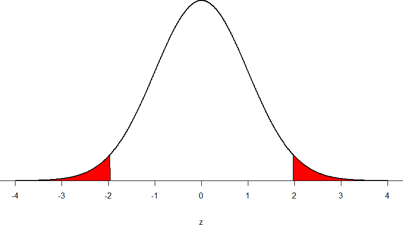
Figure 7: Rejection region for z* = ±1.96
Step 3: Calculate the Test Statistic
Now we come to our formal calculations. Let’s say that the manager collects data and finds that the average cups of this employee’s popcorn bags is ̅X = 7.75 cups. We can now plug this value, along with the values presented in the original problem, into our equation for z:
So our test statistic is z = -2.50, which we can draw onto our rejection region distribution:
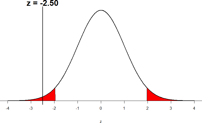
Figure 8: Test statistic location
Step 4: Make the Decision
Looking at Figure 5, we can see that our obtained z-statistic falls in the rejection region. We can also directly compare it to our critical value: in terms of absolute value, -2.50 > -1.96, so we reject the null hypothesis. We can now write our conclusion:
When we write our conclusion, we write out the words to communicate what it actually means, but we also include the average sample size we calculated (the exact location doesn’t matter, just somewhere that flows naturally and makes sense) and the z-statistic and p-value. We don’t know the exact p-value, but we do know that because we rejected the null, it must be less than α.
Effect Size
When we reject the null hypothesis, we are stating that the difference we found was statistically significant, but we have mentioned several times that this tells us nothing about practical significance. To get an idea of the actual size of what we found, we can compute a new statistic called an effect size. Effect sizes give us an idea of how large, important, or meaningful a statistically significant effect is.
For mean differences like we calculated here, our effect size is Cohen’s d:
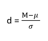
Effect sizes are incredibly useful and provide important information and clarification that overcomes some of the weakness of hypothesis testing. Whenever you find a significant result, you should always calculate an effect size
| d | Interpretation |
|---|---|
| 0.0 – 0.2 | negligible |
| 0.2 – 0.5 | small |
| 0.5 – 0.8 | medium |
| 0.8 – | large |
Table 1. Interpretation of Cohen’s d
Example: Office Temperature
Let’s do another example to solidify our understanding. Let’s say that the office building you work in is supposed to be kept at 74 degree Fahrenheit but is allowed
to vary by 1 degree in either direction. You suspect that, as a cost saving measure, the temperature was secretly set higher. You set up a formal way to test your hypothesis.
Step 1: State the Hypotheses
You start by laying out the null hypothesis:
H0: There is no difference in the average building temperature H0: μ = 74
Next you state the alternative hypothesis. You have reason to suspect a specific direction of change, so you make a one-tailed test:
HA: The average building temperature is higher than claimed HA: μ > 74
Step 2: Find the Critical Values
Step 3: Calculate the Test Statistic
Now that you have everything set up, you spend one week collecting temperature data:
|
Day |
Temp |
|
Monday |
77 |
|
Tuesday |
76 |
|
Wednesday |
74 |
|
Thursday |
78 |
|
Friday |
78 |
You calculate the average of these scores to be 𝑋̅ = 76.6 degrees. You use this to calculate the test statistic, using μ = 74 (the supposed average temperature), σ = 1.00 (how much the temperature should vary), and n = 5 (how many data points you collected):
z = 76.60 − 74.00 = 2.60 = 5.78
1.00/√5 0.45
This value falls so far into the tail that it cannot even be plotted on the distribution!
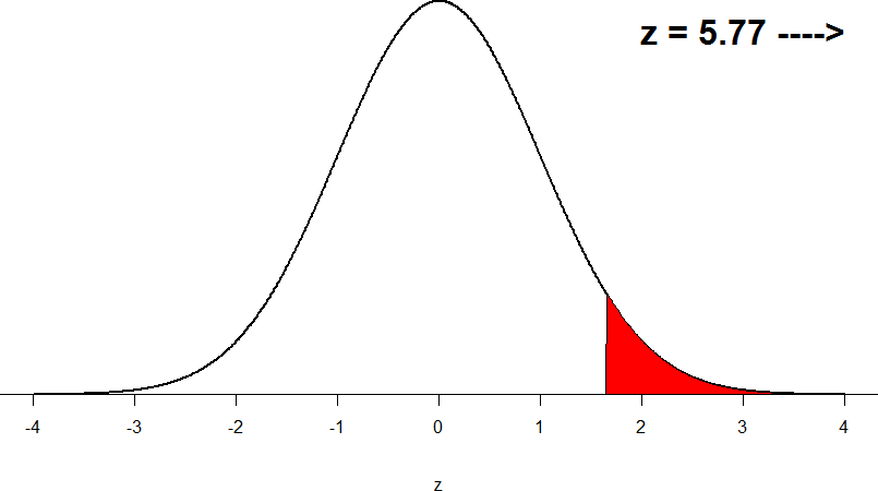
Figure 7: Obtained z-statistic
Step 4: Make the Decision
You compare your obtained z-statistic, z = 5.77, to the critical value, z* = 1.645, and find that z > z*. Therefore you reject the null hypothesis, concluding: Based on 5 observations, the average temperature (𝑋̅ = 76.6 degrees) is statistically significantly higher than it is supposed to be, z = 5.77, p < .05.
d = (76.60-74.00)/ 1= 2.60
The effect size you calculate is definitely large, meaning someone has some explaining to do!
Example: Different Significance Level
First, let’s take a look at an example phrased in generic terms, rather than in the context of a specific research question, to see the individual pieces one more time. This time, however, we will use a stricter significance level, α = 0.01, to test the hypothesis.
Step 1: State the Hypotheses
We will use 60 as an arbitrary null hypothesis value: H0: The average score does not differ from the population H0: μ = 50
We will assume a two-tailed test: HA: The average score does differ HA: μ ≠ 50
Step 2: Find the Critical Values
We have seen the critical values for z-tests at α = 0.05 levels of significance several times. To find the values for α = 0.01, we will go to the standard normal table and find the z-score cutting of 0.005 (0.01 divided by 2 for a two-tailed test) of the area in the tail, which is zcrit* = ±2.575. Notice that this cutoff is much higher than it was for α = 0.05. This is because we need much less of the area in the tail, so we need to go very far out to find the cutoff. As a result, this will require a much larger effect or much larger sample size in order to reject the null hypothesis.
Step 3: Calculate the Test Statistic
We can now calculate our test statistic. The average of 10 scores is M = 60.40 with a µ = 60. We will use σ = 10 as our known population standard deviation. From this information, we calculate our z-statistic as:
Step 4: Make the Decision
Our obtained z-statistic, z = 0.13, is very small. It is much less than our critical value of 2.575. Thus, this time, we fail to reject the null hypothesis. Our conclusion would look something like:
Notice two things about the end of the conclusion. First, we wrote that p is greater than instead of p is less than, like we did in the previous two examples. This is because we failed to reject the null hypothesis. We don’t know exactly what the p- value is, but we know it must be larger than the α level we used to test our hypothesis. Second, we used 0.01 instead of the usual 0.05, because this time we tested at a different level. The number you compare to the p-value should always be the significance level you test at. Because we did not detect a statistically significant effect, we do not need to calculate an effect size. Note: some statisticians will suggest to always calculate effects size as a possibility of Type II error. Although insignificant, calculating d = (60.4-60)/10 = .04 which suggests no effect (and not a possibility of Type II error).
Review Considerations in Hypothesis Testing
Errors in Hypothesis Testing
Keep in mind that rejecting the null hypothesis is not an all-or-nothing decision. The Type I error rate is affected by the α level: the lower the α level the lower the Type I error rate. It might seem that α is the probability of a Type I error. However, this is not correct. Instead, α is the probability of a Type I error given that the null hypothesis is true. If the null hypothesis is false, then it is impossible to make a Type I error. The second type of error that can be made in significance testing is failing to reject a false null hypothesis. This kind of error is called a Type II error.
Statistical Power
The statistical power of a research design is the probability of rejecting the null hypothesis given the sample size and expected relationship strength. Statistical power is the complement of the probability of committing a Type II error. Clearly, researchers should be interested in the power of their research designs if they want to avoid making Type II errors. In particular, they should make sure their research design has adequate power before collecting data. A common guideline is that a power of .80 is adequate. This means that there is an 80% chance of rejecting the null hypothesis for the expected relationship strength.
Given that statistical power depends primarily on relationship strength and sample size, there are essentially two steps you can take to increase statistical power: increase the strength of the relationship or increase the sample size. Increasing the strength of the relationship can sometimes be accomplished by using a stronger manipulation or by more carefully controlling extraneous variables to reduce the amount of noise in the data (e.g., by using a within-subjects design rather than a between-subjects design). The usual strategy, however, is to increase the sample size. For any expected relationship strength, there will always be some sample large enough to achieve adequate power.
Inferential statistics uses data from a sample of individuals to reach conclusions about the whole population. The degree to which our inferences are valid depends upon how we selected the sample (sampling technique) and the characteristics (parameters) of population data. Statistical analyses assume that sample(s) and population(s) meet certain conditions called statistical assumptions.
It is easy to check assumptions when using statistical software and it is important as a researcher to check for violations; if violations of statistical assumptions are not appropriately addressed then results may be interpreted incorrectly.
Learning Objectives
Having read the chapter, students should be able to:
- Conduct a hypothesis test using a z-score statistics, locating critical region, and make a statistical decision including.
- Explain the purpose of measuring effect size and power, and be able to compute Cohen’s d.
Exercises – Ch. 10
- List the main steps for hypothesis testing with the z-statistic. When and why do you calculate an effect size?
- Determine whether you would reject or fail to reject the null hypothesis in the following situations:
- z = 1.99, two-tailed test at α = 0.05
- z = 1.99, two-tailed test at α = 0.01
- z = 1.99, one-tailed test at α = 0.05
- z = 1.99, one-tailed test at α = 0.05
- You are part of a trivia team and have tracked your team’s performance since you started playing, so you know that your scores are normally distributed with μ = 78 and σ = 12. Recently, a new person joined the team, and you think the scores have gotten better. Use hypothesis testing to see if the average score has improved based on the following 8 weeks’ worth of score data: 82, 74, 62, 68, 79, 94, 90, 81, 80.
- A study examines self-esteem and depression in teenagers. A sample of 25 teens with a low self-esteem are given the Beck Depression Inventory. The average score for the group is 20.9. For the general population, the average score is 18.3 with σ = 12. Use a two-tail test with α = 0.05 to examine whether teenagers with low self-esteem show significant differences in depression.
- You get hired as a server at a local restaurant, and the manager tells you that servers’ tips are $42 on average but vary about $12 (μ = 42, σ = 12). You decide to track your tips to see if you make a different amount, but because this is your first job as a server, you don’t know if you will make more or less in tips. After working 16 shifts, you find that your average nightly amount is $44.50 from tips. Test for a difference between this value and the population mean at the α = 0.05 level of significance.
Answers to Odd- Numbered Exercises – Ch. 10
1. List hypotheses. Determine critical region. Calculate z. Compare z to critical region. Draw Conclusion. We calculate an effect size when we find a statistically significant result to see if our result is practically meaningful or important
5. Step 1: H0: μ = 42 “My average tips does not differ from other servers”, HA: μ ≠ 42 “My average tips do differ from others”
