
18 Chapter 18. Chi-square
We come at last to our final statistic: chi-square (χ2). This test is a special form of analysis called a non-parametric test, so the structure of it will look a little bit different from what we have done so far. However, the logic of hypothesis testing remains unchanged. The purpose of chi-square is to understand the frequency distribution of a single categorical variable or find a relation between two categorical variables, which is a frequently very useful way to look at our data.
Categories and Frequency Tables
Our data for the χ2 test are categorical, specifically nominal, variables. Recall from unit 1 that nominal variables have no specified order and can only be described by their names and the frequencies with which they occur in the dataset. Thus, unlike our other variables that we have tested, we cannot describe our data for the χ2 test using means and standard deviations. Instead, we will use frequencies tables.
|
|
Cat |
Dog |
Other |
Total |
|
Observed |
14 |
17 |
5 |
36 |
|
Expected |
12 |
12 |
12 |
36 |
Table 1. Pet Preferences
Table 1 gives an example of a frequency table used for a χ2 test. The columns represent the different categories within our single variable, which in this example is pet preference. The χ2 test can assess as few as two categories, and there is no technical upper limit on how many categories can be included in our variable, although, as with ANOVA, having too many categories makes our computations long and our interpretation difficult. The final column in the table is the total number of observations, or N. The χ2 test assumes that each observation comes from only one person and that each person will provide only one observation, so our total observations will always equal our sample size.
There are two rows in this table. The first row gives the observed frequencies of each category from our dataset; in this example, 14 people reported liking preferring cats as pets, 17 people reported preferring dogs, and 5 people reported a different animal. The second row gives expected values; expected values are what would be found if each category had equal representation.
The calculation for an expected value is:
E = N / C
Where N is the total number of people in our sample and C is the number of categories in our variable (also the number of columns in our table).
The expected values correspond to the null hypothesis for χ2 tests: equal representation of categories. Our first of two χ2 tests, the Goodness-of-Fit test, will assess how well our data lines up with, or deviates from, this assumption.
Goodness-of-Fit
The first of our two χ2 tests assesses one categorical variable against a null hypothesis of equally sized frequencies. Equal frequency distributions are what we would expect to get if categorization was completely random. We could, in theory, also test against a specific distribution of category sizes if we have a good reason to (e.g. we have a solid foundation of how the regular population is distributed), but this is less common, so we will not deal with it in this text.
Hypotheses
All χ2 tests, including the goodness-of-fit test, are non-parametric. This means that there is no population parameter we are estimating or testing against; we are working only with our sample data. Because of this, there are no mathematical statements for χ2 hypotheses. This should make sense because the mathematical hypothesis statements were always about population parameters (e.g. μ), so if we are non-parametric, we have no parameters and therefore no mathematical statements.
We do, however, still state our hypotheses verbally. For goodness-of-fit χ2 tests, our null hypothesis is that there is an equal number of observations in each category. That is, there is no difference between the categories in how prevalent they are. Our alternative hypothesis says that the categories do differ in their frequency. We do not have specific directions or one-tailed tests for χ2, matching our lack of mathematical statement.
Degrees of Freedom and the χ2 table
Our degrees of freedom for the χ2 test are based on the number of categories we have in our variable, not on the number of people or observations like it was for our other tests. Luckily, they are still as simple to calculate.
So for our pet preference example, we have 3 categories, so we have 2 degrees of freedom. Our degrees of freedom, along with our significance level (still defaulted to α = 0.05) are used to find our critical values in the χ2 table, which is shown in figure 1. Because we do not have directional hypotheses for χ2 tests, we do not need to differentiate between critical values for 1- or 2-tailed tests. In fact, just like our F tests for regression and ANOVA, all χ2 tests are 1-tailed tests.
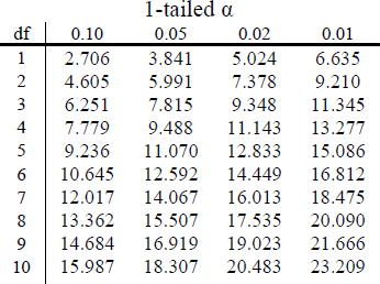
Figure 1. First 10 rows of the χ2 table
χ2 Statistic
The calculations for our test statistic in χ2 tests combine our information from our observed frequencies (O) and our expected frequencies (E) for each level of our categorical variable. For each cell (category) we find the difference between the observed and expected values, square them, and divide by the expected values. We then sum this value across cells for our test statistic.
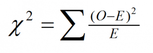
For our pet preference data, we would have:
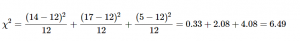
Notice that, for each cell’s calculation, the expected value in the numerator and the expected value in the denominator are the same value. Let’s now take a look at an example from start to finish.
Goodness-of-Fit Example: Pineapple on Pizza
There is a very passionate and on-going debate on whether or not pineapple should go on pizza. Being the objective, rational data analysts that we are, we will collect empirical data to see if we can settle this debate once and for all. We gather data from a group of adults asking for a simple Yes/No answer.
Step 1: State the Hypotheses
We start, as always, with our hypotheses. Our null hypothesis of no difference will state that an equal number of people will say they do or do not like pineapple on pizza, and our alternative will be that one side wins out over the other:
H0: An equal number of people do and do not like pizza.
HA: A significant majority of people will agree one way or another
Step 2: Find the Critical Value
To avoid any potential bias in this crucial analysis, we will leave α at its typical level. We have two options in our data (Yes or No), which will give us two categories. Based on this, we will have 1 degree of freedom. From our χ2 table, we find a critical value of 3.84.
Step 3: Calculate the Test Statistic
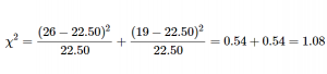
The results of the data collection are presented in table 2. We had data from 45 people in all and 2 categories, so our expected values are E = 45/2 = 22.50.
|
|
Yes |
No |
Total |
|
Observed |
26 |
19 |
45 |
|
Expected |
22.50 |
22.50 |
45 |
We can use these to calculate our χ2 statistic:
Step 4: Make the Decision
Our observed test statistic had a value of 1.08 and our critical value was 3.84. Our test statistic was smaller than our critical value, so we fail to reject the null hypothesis, and the debate rages on.
Goodness-of-Fit Example 2: Favorite candy
Our null hypothesis of no difference will state that an equal number of people select favorite candy, and our alternative will be that one type of candy is more popular:
H0: The proportion of each type of candy is equal. People have evenly distributed candy preference among our 3 choices.
HA: The proportion of each type of candy is not equal. There is an unequal distribution for candy preference.
Step 2: Find the Critical Value
To avoid any potential bias in this crucial analysis, we will leave α at its typical level. We have three options for favorite candy. Based on this, we will have 2 degree of freedom. From our χ2 table, we find a critical value of 5.99.
Step 3: Calculate Statistic
The results of the data collection are presented in table 3. We had data from 100 people in all and 3 categories, so our expected values are E = 100/3 = 33.333.
| Candy Type | Count | Expected | (O-E)2 |
|---|---|---|---|
| chocolate | 30 | 33.333 | 11.11 |
| licorice | 33 | 33.333 | 0.11 |
| gumball | 37 | 33.333 | 13.44 |
Table 3 Observed and expected counts for candy data
Step 4: Make the Decision
For the candy example, the observed counts of candies are not particularly surprising based on the proportions printed on the bag of candy, and we would not reject the null hypothesis of equal proportions.
Contingency Tables for Two Variables
|
College Sports |
Affected Decision |
|
|||
|
Primary |
Somewhat |
No |
Total |
||
|
Watched |
Yes |
47 |
26 |
14 |
87 |
|
No |
21 |
23 |
37 |
81 |
|
|
|
Total |
68 |
49 |
51 |
168 |
Table 3. Contingency table of college sports and decision making
In contrast to the frequency table for our goodness-of-fit test, our contingency table does not contain expected values, only observed data. Within our table, wherever our rows and columns cross, we have a cell. A cell contains the frequency of observing it’s corresponding specific levels of each variable at the same time. The top left cell in table 3 shows us that 47 people in our study watched college sports as a child AND had college sports as their primary deciding factor in which college to attend.
Cells are numbered based on which row they are in (rows are numbered top to bottom) and which column they are in (columns are numbered left to right). We always name the cell using (R,C), with the row first and the column second. A quick and easy way to remember the order is that R/C Cola exists but C/R Cola does not. Based on this convention, the top left cell containing our 47 participants who watched college sports as a child and had sports as a primary criteria is cell (1,1). Next to it, which has 26 people who watched college sports as a child but had sports only somewhat affect their decision, is cell (1,2), and so on. We only number the cells where our categories cross. We do not number our total cells, which have their own special name: marginal values. Marginal values are the total values for a single category of one variable, added up across levels of the other variable. In table 3, these marginal values have been italicized for ease of explanation, though this is not normally the case. We can see that, in total, 87 of our participants (47+26+14) watched college sports growing up and 81 (21+23+37) did not. The total of these two marginal values is 168, the total number of people in our study. Likewise, 68 people used sports as a primary criteria for deciding which college to attend, 50 considered it somewhat, and 50 did not use it as criteria at all. The total of these marginal values is also 168, our total number of people. The marginal values for rows and columns will always both add up to the total number of participants, N, in the study. If they do not, then a calculation error was made and you must go back and check your work.
Expected Values of Contingency Tables
Our expected values for contingency tables are based on the same logic as they were for frequency tables, but now we must incorporate information about how frequently each row and column was observed (the marginal values) and how many people were in the sample overall (N) to find what random chance would have made the frequencies out to be.
Expected values formula
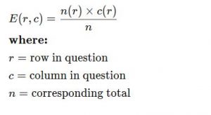
The subscripts n(r) is the count for the row and n(c) the count for the column, respectively, correspond to the cell we are calculating the expected frequency for, and n is still the total sample size.
Example: Using the data from table 3, we can calculate the expected frequency for cell, E(1,1), the college sport watchers who used sports at their primary criteria, is
E(1,1) = (87)(68) / 168 = 35.21
|
College Sports |
Affected Decision |
|
|||
|
Primary |
Somewhat |
No |
Total |
||
|
Watched |
Yes |
47 |
26 |
14 |
87 |
|
No |
21 |
23 |
37 |
81 |
|
|
|
Total |
68 |
49 |
51 |
168 |
We can follow the same math to find all the expected values for this table:
|
Expected Values |
Affected Decision |
|
|||
|
Primary |
Somewhat |
No |
Total |
||
|
Watched |
Yes |
35.21 |
25.38 |
26.41 |
87 |
|
No |
32.79 |
23.62 |
24.59 |
81 |
|
|
|
Total |
68 |
49 |
51 |
|
Table 4. Expected Values derived from Table 3.
Notice that the marginal values still add up to the same totals as before. This is because the expected frequencies are just row and column averages simultaneously. Our total N will also add up to the same value.
Test for Independence
The χ2 test performed on contingency tables is known as the test for independence. In this analysis, we are looking to see if the values of each categorical variable (that is, the frequency of their levels) is related to or independent of the values of the other categorical variable. Because we are still doing a χ2 test, which is non- parametric, we still do not have mathematical versions of our hypotheses. The actual interpretations of the hypotheses are quite simple: the null hypothesis says that the variables are independent or not related, and alternative says that they are not independent or that they are related. For step 2, the only change is degrees of formula. Our critical value will come from the same table that we used for the goodness-of- fit test, but our degrees of freedom will change. Because we now have rows and columns (instead of just columns) our new degrees of freedom.
For step 3, we still use the χ2 but we need to compute expected frequencies. Step 4 is the same process. Let’s see an example.
Example: College Sports
Step 1: Hypotheses
Step 3: Calculate the Test Statistic
The same formula for χ2 is used once again. We are using the expected frequency values from table 4:
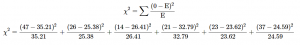 = 3.94 + 0.02 + 5.83 + 4.24 + 0.02 + 6.26 = 20.31
Reject H0. Based on our data from 168 people, we can say that there is a statistically significant relation between whether or not someone watches college sports growing up and how much a college’s sports team factor in to that person’s decision on which college to attend, χ2(2) = 20.31, p < 0.05.
Effect Size for χ2
Like all other significance tests, χ2 tests – both goodness-of-fit and tests for independence – have effect sizes that can and should be calculated for statistically significant results. There are many options for which effect size to use, and the ultimate decision is based on the type of data, the structure of your frequency or contingency table, and the types of conclusions you would like to draw. For the purpose of our introductory course, we will focus only on a single effect size that is simple and flexible: Cramer’s V.
Cramer’s V formula 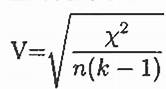 For this calculation, k is the smaller value of either R (the number of rows) or C (the number of columns). The numerator is simply the test statistic (χ2) we calculate during step 3 of the hypothesis testing procedure.
Example Continued: College Sports
Effect size
For our example, we had 2 rows and 3 columns, so k = 2:
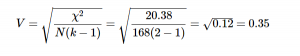
So the statistically significant relation between our variables was moderately strong examining the effect size table below.
Like other statistic effect sizes there are range cut offs of small, medium, and large. The effect size ranges of Cramer’s V are in Table 6.
| small | medium | large | |
| df = 1 | 0.10 | 0.30 | 0.50 |
| df = 2 | 0.07 | 0.21 | 0.35 |
| df = 3 | 0.06 | 0.17 | 0.29 |
Beyond Pearson’s Chi-Square Test: Standardized Residuals
For a more applicable example, let’s take the question of whether a Black driver is more likely to be searched when they are pulled over by a police officer, compared to a white driver. The Stanford Open Policing Project (https://openpolicing.stanford.edu/) has studied this, and provides data that we can use to analyze the question. We will use the data from the State of Connecticut since they are fairly small and thus easier to analyze.
The standard way to represent data from a categorical analysis is through a contingency table, which presents the number or proportion of observations falling into each possible combination of values for each of the variables. Table 6 below shows the contingency table for the police search data. It can also be useful to look at the contingency table using proportions rather than raw numbers, since they are easier to compare visually, so we include both absolute and relative numbers here.
| searched | Black | White | Black (relative) | White (relative) |
|---|---|---|---|---|
| FALSE | 36244 | 239241 | 0.13 | 0.86 |
| TRUE | 1219 | 3108 | 0.00 | 0.01 |
Table 6. Contigency Table for Police Search Data
The Pearson chi-squared test (discussed above) allows us to test whether observed frequencies are different from expected frequencies, so we need to determine what frequencies we would expect in each cell if searches and race were unrelated – which we can define as being independent. If we perform this test easily using our statistical software, X2 (1) = 828, p < .001. This shows that the observed data would be highly unlikely if there was truly no relationship between race and police searches, and thus we should reject the null hypothesis of independence.
When we find a significant effect with the chi-squared test, this tells us that the data are unlikely under the null hypothesis, but it doesn’t tell us how the data differ. To get a deeper insight into how the data differ from what we would expect under the null hypothesis, we can examine the residuals from the model, which reflects the deviation of the data (i.e., the observed frequencies) from the model (i.e., the expected frequencies) in each cell. Rather than looking at the raw residuals (which will vary simply depending on the number of observations in the data), it’s more common to look at the standardized residuals (sometimes called Pearson residuals).
Table 7 shows these for the police stop data from X2 above. Remember that we examined the question of whether a Black driver is more likely to be searched when they are pulled over by a police officer, compared to a white driver. These standardized residuals can be interpreted as Z scores – in this case, we see that the number of searches for Black individuals are substantially higher than expected based on independence, and the number of searches for white individuals are substantially lower than expected. This provides us with the context that we need to interpret the significant chi-squared result.
| searched | driver_race | Standardized residuals |
|---|---|---|
| FALSE | Black | -3.3 |
| TRUE | Black | 26.6 |
| FALSE | White | 1.3 |
| TRUE | White | -10.4 |
Table 7. Summary of standardized residuals for police stop data
Beware of Simpson’s paradox
The contingency tables that represent summaries of large numbers of observations, but summaries can sometimes be misleading. Let’s take an example from baseball. The table below shows the batting data (hits/at bats and batting average) for Derek Jeter and David Justice over the years 1995-1997:
| Player | 1995 | 1996 | 1997 | Combined | ||||
|---|---|---|---|---|---|---|---|---|
| Derek Jeter | 12/48 | .250 | 183/582 | .314 | 190/654 | .291 | 385/1284 | .300 |
| David Justice | 104/411 | .253 | 45/140 | .321 | 163/495 | .329 | 312/1046 | .298 |
Table 9. Player Batting data for 2 baseball players
If you look closely, you will see that something odd is going on: In each individual year Justice had a higher batting average than Jeter, but when we combine the data across all three years, Jeter’s average is actually higher than Justice’s! This is an example of a phenomenon known as Simpson’s paradox, in which a pattern that is present in a combined dataset may not be present in any of the subsets of the data. This occurs when there is another variable that may be changing across the different subsets – in this case, the number of at-bats varies across years, with Justice batting many more times in 1995 (when batting averages were low). We refer to this as a lurking variable, and it’s always important to be attentive to such variables whenever one examines categorical data.
Learning objectives
Having read the chapter, a student should be able to:
- Identify when appropriate to run a chi-square test of goodness-of-fit or independence.
- Describe the concept of a contingency table for categorical data.
- Compute it for a given contingency table.
- Complete hypothesis test for chi-square test of goodness-of-fit and independence.
- Compute and interpret effect size for chi-square chi-square test of goodness-of-fit or independence.
- Describe Simpson’s paradox and why it is important for categorical data analysis.
Exercises – Ch. 18
- What does a frequency table display? What does a contingency table display?
2. What does a goodness-of-fit test assess?
3. How do expected frequencies relate to the null hypothesis?
4. What does a test-for-independence assess?
5. Compute the expected frequencies for the following contingency table:
|
|
Category A |
Category B |
|
Category C |
22 |
38 |
|
Category D |
16 |
14 |
6. Test significance and find effect sizes (if significant) for the following tests:
- N = 19, R = 3, C = 2, χ2 (2) = 7.89, α = .05
- N = 12, R = 2, C = 2, χ2 (1) = 3.12, α = .05
- N = 74, R = 3, C = 3, χ2 (4) = 28.41, α = .01
7. You hear a lot of people claim that The Empire Strikes Back is the best movie in the original Star Wars trilogy, and you decide to collect some data to demonstrate this empirically (pun intended). You ask 48 people which of the original movies they liked best; 8 said A New Hope was their favorite, 23 said The Empire Strikes Back was their favorite, and 17 said Return of the Jedi was their favorite. Perform a chi-square test on these data at the .05 level of significance.
8. A pizza company wants to know if people order the same number of different toppings. They look at how many pepperoni, sausage, and cheese pizzas were ordered in the last week; fill out the rest of the frequency table and test for a difference.
|
|
Pepperoni |
Sausage |
Cheese |
Total |
|
Observed |
320 |
275 |
251 |
|
|
Expected |
|
|
|
|
9. A university administrator wants to know if there is a difference in proportions of students who go on to grad school across different majors. Use the data below to test whether there is a relation between college major and going to grad school.
|
|
Major |
|||
|
Psychology |
Business |
Math |
||
|
Graduate School |
Yes |
32 |
8 |
36 |
|
No |
15 |
41 |
12 |
|
10.A company you work for wants to make sure that they are not discriminating against anyone in their promotion process. You have been asked to look across gender to see if there are differences in promotion rate (i.e. if gender and promotion rate are independent or not). The following data should be assessed at the normal level of significance:
|
|
Promoted in last two years? |
||
|
Yes |
No |
||
|
Gender |
Women |
8 |
5 |
|
Men |
9 |
7 |
|
Answers to Odd- Numbered Exercises – Ch. 18
1. Frequency tables display observed category frequencies and (sometimes) expected category frequencies for a single categorical variable. Contingency tables display the frequency of observing people in crossed category levels for two categorical variables, and (sometimes) the marginal totals of each variable level.
|
Observed |
Category A |
Category B |
Total |
|
Category C |
22 |
38 |
60 |
|
Category D |
16 |
14 |
30 |
|
Total |
38 |
52 |
90 |
|
Expected |
Category A |
Category B |
Total |
|
Category C |
((60*38)/90) = 25.33 |
((60*52)/90) = 34.67 |
60 |
|
Category D |
((30*38)/90) = 12.67 |
((30*52)/90) = 17.33 |
30 |
|
Total |
38 |
52 |
90 |
7. Step 1: H0: “There is no difference in preference for one movie”, HA: “There is a difference in how many people prefer one movie over the others.” Step 2: 3 categories (columns) gives df = 2, χ2crit = 5.991. Step 3: Based on the given frequencies:
|
|
New Hope |
Empire |
Jedi |
Total |
|
Observed |
8 |
23 |
17 |
48 |
|
Expected |
16 |
16 |
16 |
|
χ2 = 7.13. Step 4: Our obtained statistic is greater than our critical value, reject H0. Based on our sample of 48 people, there is a statistically significant difference in the proportion of people who prefer one Star Wars movie over the others, χ2(2) = 7.13, p < .05. Since this is a statistically significant result, we should calculate an effect size: Cramer’s V = √ 7.13/48(3−1) = 0.27, which is a moderate effect size.
|
Expected Values |
Major |
|||
|
Psychology |
Business |
Math |
||
|
Graduate School |
Yes |
24.81 |
25.86 |
25.33 |
|
No |
22.19 |
23.14 |
22.67 |
|
χ2 = 2.09+12.34+4.49+2.33+13.79+5.02 = 40.05. Step 4: Obtained statistic is greater than the critical value, reject H0. Based on our data, there is a statistically significant relation between college major and going to grad school, χ2(2) = 40.05, p < .05, Cramer’s V = 0.53, which is a large effect.
