
5 Chapter 5: Measures of Dispersion
Measure of central tendency (a value around which other scores in the set cluster) and a measure of variability (an indicator of how spread out about the mean scores are in a data set) are used together to give a description of the data.
The terms variability, spread, and dispersion are synonyms, and refer to how spread out a distribution is. Just as in the section on central tendency where we discussed measures of the center of a distribution of scores, in this chapter we will discuss measures of the variability of a distribution.
Measures of dispersion describe the spread of scores in a distribution. The more spread out the scores are, the higher the dispersion or spread. In Figure 1, the y-axis is frequency and the x-axis represents values for a variable. There are two distributions, labeled as small and large. You can see both are normally distributed (unimodal, symmetrical), and the mean, median, and mode for both fall on the same point. What is different between the two is the spread or dispersion of the scores. The taller-looking distribution shows a smaller dispersion while the wider distribution shows a larger dispersion. For the “small” distribution in Figure 1, the data values are concentrated closely near the mean; in the “large” distribution, the data values are more widely spread out from the mean.
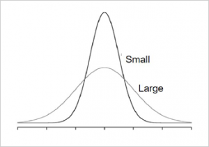
Figure 1. Examples of 2 normal (symmetrical, unimodal) distributions.
In this chapter, we will look at three measures of variability: range, variance, and standard deviation. An important characteristic of any set of data is the variation in the data. Imagine that students in two different sections of statistics take Exam 1 and the mean score in both classrooms is a 75. If that is the only descriptive statistic I report you might assume that both classes are identical – but that is not necessarily true. Let’s examine the scores for each section.
| Section A | Section B |
| Scores = 70, 70, 70, 70, 85, 85
Mean = 75 |
Scores = 70, 72, 73, 75, 75, 85
Mean = 75 |
Table 1. Exam scores for 2 sections of a class.
Comparing both sections you can see that the scores for Section A very few scores are represented (e.g., 70 and 85) and they are very far from the mean, while in Section B more scores are represented and clustered close to the mean We would say that the spread of scores for Section A is greater than Section B.
Range
The range is the simplest measure of variability and is really easy to calculate.
You can see in our statistics course example (Table 1) that Section A scores have a range of 15 and Section B scores have a range of 15. That means all the other scores are not included and may not give an unbiased description of the data.
The range is the simplest measure of variability to calculate, and one you have probably encountered many times in your life. The simplicity of calculating range is appealing but it can be a very unreliable measure of variability. We noticed earlier that the spread of score for each section was very different for each section.
Let’s take a few examples. What is the range of the following group of numbers: 10, 2, 5, 6, 7, 3, 4? Well, the highest number is 10, and the lowest number is 2, so 10 – 2 = 8. The range is 8. Let’s take another example. Here’s a dataset with 10 numbers: 99, 45, 23, 67, 45, 91, 82, 78, 62, 51. What is the range? The highest number is 99 and the lowest number is 23, so 99 – 23 equals 76; the range is 76. Again, the problem with using range is that it is extremely sensitive to outliers, and one number far away from the rest of the data will greatly alter the value of the range. For example, in the set of numbers 1, 3, 4, 4, 5, 8, and 9, the range is 8 (9 – 1). However, if we add a single person whose score is nowhere close to the rest of the scores, say, 20, the range more than doubles from 8 to 19.
Interquartile Range
A special take on range, is to identify values in terms of quartiles of the distribution (remember chapter 2 with boxplots). The interquartile range (IQR) is the range of the middle 50% of the scores in a distribution and is sometimes used to communicate where the bulk of the data in the distribution are located. It is computed as follows: IQR = 75th percentile – 25th percentile. Recall that in the discussion of box plots in chapter 2, the 75th percentile was called the upper hinge and the 25th percentile was called the lower hinge. Using this terminology, the interquartile range is referred to as the H-spread.
The Mean Needed to Further Examine Dispersion
Variability can also be defined in terms of how close the scores in the distribution are to the middle of the distribution. Using the mean as the measure of the center of the distribution, we can see how far, on average, each data point is from the center. Remember that the mean is the point on which a distribution would balance. We can examine spread by identifying how far each value is from the mean. This is known as the deviation from the mean (or differences from the mean). The sum of deviations is the smallest for the mean value. Interestingly, the sum of deviation from the mean is zero because the mean is the fulcrum or balance point.
Let’s revisit an example from chapter 4 (Figure 2). We had a set of 5 numbers: 2, 3, 4, 9, and 16 with a mean of 6.8.
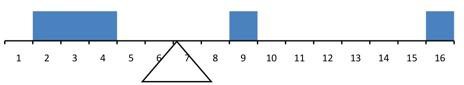
Figure 2. The distribution balances at the mean of 6.8.
In Table 2, the value is represented as X, the column “deviation from the mean or 𝑋 − mean” contains deviations (how far each score deviates from the mean), here calculated as the score minus 6.8.
|
Value (X) |
Deviation from the Mean (X – mean) |
|
2 |
-4.8 |
|
3 |
-3.8 |
|
4 |
-2.8 |
|
9 |
2.2 |
| 16 |
9.2 |
|
Total (Σ ) |
0 |
Table 2 (from chapter 4) shows the deviations of the numbers 2, 3, 4, 9, and 16 from their mean of 6.8.
Moving toward variance: sum of squares deviations
For us to get to a value that would represent the dispersion, we will add another step from calculating the deviation of the mean scores. You can see in Table 3 there is now a third column, the squared deviations column. The column “(𝑋 − mean)2” has the “Squared Deviations” and is simply the previous column squared.
|
Value (X) |
Deviation from the Mean (X – mean) |
Squared Deviations (X-mean)2 |
|
2 |
-4.8 | 23.04 |
|
3 |
-3.8 | 14.44 |
|
4 |
-2.8 | 7.84 |
|
9 |
2.2 | 4.84 |
| 16 | 9.2 | 84.64 |
|
Total (Σ ) |
0 | 134.8 (←Sum of Squares/SS) |
Table 3. Adding on a squared deviations column to create “sum of squares” or SS
Here is another example of calculating SS with 20 data points where the mean = 7:
| X | X − mean | (X − mean)2 |
|
9 |
2 |
4 |
|
9 |
2 |
4 |
|
9 |
2 |
4 |
|
8 |
1 |
1 |
|
8 |
1 |
1 |
|
8 |
1 |
1 |
|
8 |
1 |
1 |
|
7 |
0 |
0 |
|
7 |
0 |
0 |
|
7 |
0 |
0 |
|
7 |
0 |
0 |
|
7 |
0 |
0 |
|
6 |
-1 |
1 |
|
6 |
-1 |
1 |
|
6 |
-1 |
1 |
|
6 |
-1 |
1 |
|
6 |
-1 |
1 |
|
6 |
-1 |
1 |
|
5 |
2 |
4 |
|
5 |
2 |
4 |
|
total (Σ ) |
Σ = 0 |
Σ = 30 |
Table 4. Calculations for Sum of Squares.
Variance
Now that we have the Sum of Squares calculated, we can use it to compute our formal measure of average distance from the mean, the variance. Informally, it measures how far a set of (random) numbers are spread out from their average value. The variance is defined as the average squared difference of the scores from the mean. The mathematical definition of the variance is the sum of the squared deviations (distances) of each score from the mean divided by the number of scores in the data set. Remember that we square the deviation scores because, as we saw in the Sum of Squares table, the sum of raw deviations is always 0, and there’s nothing we can do mathematically without changing that.
Variance
The population parameter for variance is σ2 (“sigma-squared”) and is calculated as:
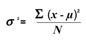
Example from Table 3: If we assume that the values in Table 3 represent the full population, then we can take our value of Sum of Squares and divide it by N to get our population variance:
σ2 = 134.8/5 = 26.96
Example from Table 4: If we assume that the values in Table 4 represent the full population, then we can take our value of Sum of Squares and divide it by N to get our population variance:
σ2 = 30/20 = 1.5
Notice that the numerator formula is identical to the formula for the Sum of Squares presented in Tables 3 and 4 with the mean replaced by μ. Thus, we can use the Sum of Squares table to easily calculate the numerator then simply divide that value by N to get variance. Remember variance for a population is noted as σ2 (sigma-squared). So, on average, scores in this population from our quiz example in Table 4 are 1.5 squared units away from the mean. Variance as a measure of spread is much more robust (a term used by statisticians to mean resilient or resistant to outliers) than the range, so it is a much more useful value to compute. Additionally, as we will see in future chapters, variance plays a central role in inferential statistics.
Variance
The sample statistic used to estimate the variance is s2 (“s-squared”):
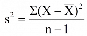
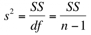
Note: the sum of square deviations is abbreviated at SS and the degrees of freedom abbreviated as df. The shorthand for sample variance is SS/df.
Example from Table 3: If we assume that the values in Table 4 represent a sample, then we can take our value of Sum of Squares and divide it by n-1 to get our sample variance:
s2 = 134.8/(5-1) = 33.7
Example from Table 4 (treating those scores as a sample): we can estimate the sample variance as:
s2 =30/(20 − 1) = 1.58
Notice that the sample variance values are slightly larger than the one we calculated when we assumed these scores were the full population. This is because our value in the denominator is slightly smaller, making the final value larger. In general, as your sample size n gets bigger, the effect of subtracting 1 becomes less and less.
Comparing a sample size of 10 to a sample size of 1000; 10 – 1 = 9, or 90% of the original value, whereas 1000 – 1 = 999, or 99.9% of the original value. Thus, larger sample sizes will bring the estimate of the sample variance closer to that of the population variance. This is a key idea and principle in statistics that we will see over and over again: larger sample sizes better reflect the population.The variance is “the sum of the squared distances of each score from the mean divided by total scores,” according to the definitional formula. This means the final answer is always in the original units of measurement, squared. This means that if we had been measuring reaction time, the units would have been seconds squared. If we had been measuring height, the units would have been inches squared. These units are not very useful because we do not talk about inches squared in day to day language.
Standard Deviation
The standard deviation is simply the square root of the variance. This is a useful and interpretable statistic because taking the square root of the variance (recalling that variance is the average squared difference) puts the standard deviation back into the original units of the measure we used. Thus, when reporting descriptive statistics in a study, scientists virtually always report mean and standard deviation. Standard deviation is therefore the most commonly used measure of spread for our purposes.
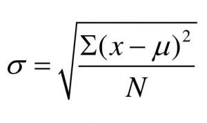
The population parameter for standard deviation is σ (“sigma”), which, intuitively, is the square root of the variance parameter σ2 (on occasion, the symbols work out nicely that way). The formula is simply the formula for variance under a square root sign.
Standard Deviation
population standard deviation is given as σ :
Example from Table 3 (data represent the full population):
σ = √(134.8/5) = √26.96 = 5.19
Example from table 4 (data represent the full population):
σ = √(30/20) = √1.5 = 1.22
The sample statistic follows the same conventions and is given as s. It is the square root of the sample variance.
Standard Deviation
sample standard deviation is given as s:
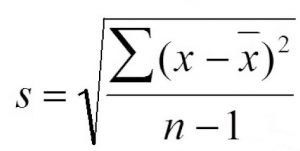
It can be noted shorthand as s = sqrt(SS/df)
Example from Table 3 (treat as sample):
s2 = 134.8/(5-1) = 33.7 so then s = sqrt(33.7) = 5.8
Example from Table 4 (treating those scores as a sample):
s2 =30/(20 − 1) = 1.58 so then s = sqrt(1.58) = 1.26
The Normal Distribution and Standard Deviation
The standard deviation is an especially useful measure of variability when the distribution is normal or approximately normal because the proportion of the distribution within a given number of standard deviations from the mean can be calculated.
For a normal distribution,
- Approximately 68% of the data is within one standard deviation of the mean.
- Approximately 95% of the data is within two standard deviations of the mean.
- More than 99% of the data is within three standard deviations of the mean.
This is known as the Empirical Rule or the 68-95-99 Rule, as shown in Figure 3.
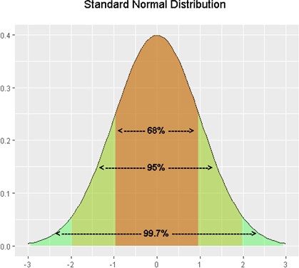
Figure 3: Percentages of the normal distribution showing the 68-95-99 rule.
Figure 4 shows two normal distributions. The red distribution has a mean of 40 and a standard deviation of 5; the blue distribution has a mean of 60 and a standard deviation of 10. For the red distribution, 68% of the distribution is between 45 and 55; for the blue distribution, 68% is between 50 and 70. Notice that as the standard deviation gets smaller, the distribution becomes much narrower, regardless of where the center of the distribution (mean) is. Figure 5 presents several more examples of this effect.
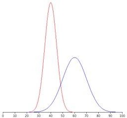
Figure 4. Normal distributions with standard deviations of 5 and 10.
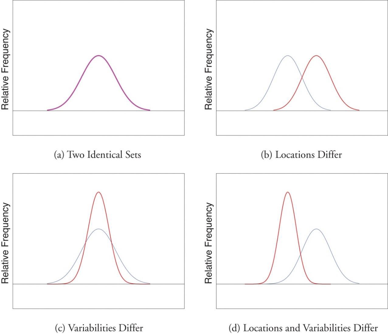
Figure 5. Differences between two datasets.
The image below represents IQ scores as measured by the Wechsler Intelligence test and has a µ = 100 and σ = 15. This means that about 70% of the scores are between 85 and 115 and that 95% of the scores are between 70 and 130.
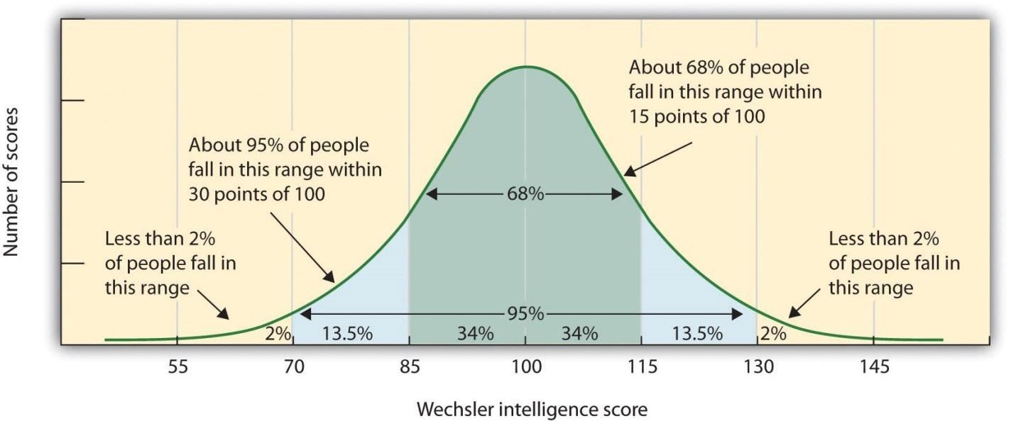
Figure 6. Weshcler IQ Score distribution. Photo credit
A data value that is two standard deviations from the average is just on the borderline for what many statisticians would consider to be far from the average, and can define outside two standard deviations as an outlier (extreme score). Considering data to be far from the mean if it is more of an approximate “rule of thumb” than a rigid rule. Some researchers may define an outlier as greater than 3 standard deviations from the mean. In general, the shape of the distribution of the data affects how much of the data is further away than two standard deviations.
Example
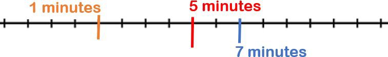
Let’s use an example to help us understand how we can use standard deviation. Suppose that we are studying the amount of time customers wait in line at the checkout at supermarket A and supermarket B.
The average wait time at both supermarkets is five minutes. At supermarket A, the standard deviation for the wait time is two minutes. At supermarket B the standard deviation for the wait time is four minutes
Because supermarket B has a higher standard deviation, we know that there is more variation in the wait times at supermarket B. Overall, wait times at supermarket B are more spread out from the average; wait times at supermarket A are more concentrated near the average.
Suppose that Rosa and Binh both shop at supermarket A. Rosa waits at the checkout counter for seven minutes and Binh waits for one minute. Rosa waits for seven minutes – Seven is two minutes longer than the average of five; two. Binh waits for one minute – One is four minutes less than the average of five; four minutes is equal to two standard deviations.
A data value that is two standard deviations from the average is just on the borderline for what many statisticians would consider to be an outlier. Again, we would also want to do more about the distributions for this data.
Recap
|
Formula for Sum of Squares for population (using μ) |
Symbol |
Meaning |
|
|
X |
Raw score |
|
X – µ |
Deviation score that is calculated by subtracting raw scores from population mean |
|
|
(X – µ )² |
The deviation scores are squared |
|
|
∑(X – µ )² |
The squared deviation scores are added up to calculate sum of squares |
|
The formula for variance expresses the mathematical definition in symbols. Recall that the symbol for the variance (like any statistic) changes depending on whether the statistic is referring to a sample or a population. Although the variance is itself a measure of variability, it generally plays a larger role in inferential statistics than in descriptive statistics.
|
Formulas |
|
|
Sample variance (s2) |
Population variance (σ2) |
|
SS/df Note: sample df = n-1 |
SS/N
|
The standard deviation is the most commonly used measure of variability because it includes all the scores of the data set in the calculation, and it is reported in the original units of measurement. It tells us the average (or standard) distance of each score from the mean of the distribution.
|
Sample Standard Deviation (s) |
Population Standard Deviation (σ) |
|
√SS/df |
√SS/N |
The standard deviation is always positive or zero. The standard deviation is small when the data are all concentrated close to the mean, exhibiting little variation or spread. The standard deviation is larger when the data values are more spread out from the mean, exhibiting more variation.
It is important to note that the Empirical Rule or the 68-95-99 rule only applies when the shape of the distribution of the data is bell-shaped and symmetric.
Factors Affecting Variability
Before we close out the chapter, we wanted to make you aware that there are several things that can impact the spread of scores.
Extreme Scores. Range is affected most by extreme scores or outliers but standard deviation and variance are also affected by extremes because they are based on squared deviations. One extreme score can have a disproportionate effect on the overall statistic or parameter.
Sample size. Increased sample size is associated with an increase in range because of the potential to increase or decrease values in a set of data.
Stability under sampling. If you take multiple samples from the same population you expect similar values because the samples come from the same source. This accounts for their stability and we would expect samples to have the same variability as the population from which it was selected.
Learning Objectives
Having read this chapter, you should be able to:
- Explain the purpose of measuring variability and differences between scores with high versus low variability
- Define and calculate measures of spread/dispersion: range, variance, standard deviation for sample and for population
- Define and calculate sum of squared deviations (SS)
Exercises – Ch. 5
1. Compute the population standard deviation for the following scores (remember to use the Sum of Squares table and this is the same data from chapter 4):
5, 7, 8, 3, 4, 4, 2, 7, 1, 6
2. For the following problem, use the following scores: 5, 8, 8, 8, 7, 8, 9, 12, 8, 9, 8, 10, 7, 9, 7, 6, 9, 10, 11, 8
3. Compute the range, sample variance, and sample standard deviation for the following scores: 25, 36, 41, 28, 29, 32, 39, 37, 34, 34, 37, 35, 30, 36, 31, 31 (same data from chapter 4)
4. Using the same values from problem 3, calculate the range, sample variance, and sample standard deviation, but this time include 65 in the list of values. How did each of the three values change?
5. Two normal distributions have exactly the same mean, but one has a standard deviation of 20 and the other has a standard deviation of 10. How would the shapes of the two distributions compare?
6. Compute the sample standard deviation for the following scores: -8, -4, -7, -6, -8, -5, -7, -9, -2, 0 (same data from chapter 4)
Answers to Odd-Numbered Exercises – Ch. 5
1. (μ = 4.80) σ2 = 2.36
3. range = 16, s2 = 18.40, s = 4.29
5. If both distributions are normal, then they are both symmetrical, and having the same mean causes them to overlap with one another. The distribution with the standard deviation of 10 will be narrower than the other distribution
