
8 Chapter 8: Sampling Distributions
People, Samples, and Populations
Most of what we have dealt with so far has concerned individual scores grouped into samples, with those samples being drawn from and, hopefully, representative of a population. We saw how we can understand the location of individual scores within a sample’s distribution via z-scores, and how we can extend that to understand how likely it is to observe scores higher or lower than an individual score via probability.
All of these principles carry forward from scores within samples to samples within populations. Just like an individual score will differ from its mean, an individual sample mean will differ from the true population mean. We encountered this principle in earlier chapters: sampling error. As mentioned way back in chapter 1, sampling error is an incredibly important principle. We know ahead of time that if we collect data and compute a sample, the observed value of that sample will be at least slightly off from what we expect it to be based on our supposed population mean; this is natural and expected. However, if our sample mean is extremely different from what we expect based on the population mean, there may be something going on.
Sampling
One of the foundational ideas in statistics is that we can make inferences about an entire population based on a relatively small sample of individuals from that population. In this chapter, we will introduce the concept of statistical sampling and discuss why it works.
Anyone living in the United States will be familiar with the concept of sampling from the political polls that have become a central part of our electoral process. In some cases, these polls can be incredibly accurate at predicting the outcomes of elections. The best known example comes from the 2008 and 2012 US Presidential elections when the pollster Nate Silver correctly predicted electoral outcomes for 49/50 states in 2008 and for all 50 states in 2012. Silver did this by combining data from 21 different polls, which vary in the degree to which they tend to lean towards either the Republican or Democratic side. Each of these polls included data from about 1000 likely voters – meaning that Silver was able to almost perfectly predict the pattern of votes of more than 125 million voters using data from only about 21,000 people, along with other knowledge (such as how those states have voted in the past).
How do we sample?
Our goal in sampling is to determine the value of a statistic for an entire population of interest, using just a small subset of the population. We do this primarily to save time and effort – why go to the trouble of measuring every individual in the population when just a small sample is sufficient to accurately estimate the statistic of interest?
In the election example, the population is all registered voters in the region being polled, and the sample is the set of 1000 individuals selected by the polling organization. The way in which we select the sample is critical to ensuring that the sample is representative of the entire population, which is a main goal of statistical sampling. It’s easy to imagine a non-representative sample; if a pollster only called individuals whose names they had received from the local Democratic party, then it would be unlikely that the results of the poll would be representative of the population as a whole. In general, we would define a representative poll as being one in which every member of the population has an equal chance of being selected. When this fails, then we have to worry about whether the statistic that we compute on the sample is biased – that is, whether its value is systematically different from the population value (which we refer to as a parameter). Keep in mind that we generally don’t know this population parameter, because if we did then we wouldn’t need to sample! But we will use examples where we have access to the entire population, in order to explain some of the key ideas.
It’s important to also distinguish between two different ways of sampling: with replacement versus without replacement. In sampling with replacement, after a member of the population has been sampled, they are put back into the pool so that they can potentially be sampled again. In sampling without replacement, once a member has been sampled they are not eligible to be sampled again. It’s most common to use sampling without replacement.
Sampling error
Regardless of how representative our sample is, it’s likely that the statistic that we compute from the sample is going to differ at least slightly from the population parameter. We refer to this as sampling error. If we take multiple samples, the value of our statistical estimate will also vary from sample to sample; we refer to this distribution of our statistic across samples as the sampling distribution.
Sampling error is directly related to the quality of our measurement of the population. Clearly, we want the estimates obtained from our sample to be as close as possible to the true value of the population parameter. However, even if our statistic is unbiased (that is, we expect it to have the same value as the population parameter), the value for any particular estimate will differ from the population value, and those differences will be greater when the sampling error is greater. Thus, reducing sampling error is an important step towards better measurement.
Until now we used z-scores and probability we were only looking for the probability of finding one score (n = 1) but most research involves looking at larger samples. Using samples allows us to make generalizations to the larger population but there are some limitations. We know that the samples will look different even when they come from the same population and the difference between the sample and population is known as sampling error.
Suppose you randomly sampled 10 people from the population of women in Houston, Texas, between the ages of 21 and 35 years and computed the mean height of your sample. You would not expect your sample mean to be equal to the mean of all women in Houston. It might be somewhat lower or it might be somewhat higher, but it would not equal the population mean exactly. Similarly, if you took a second sample of 10 people from the same population, you would not expect the mean of this second sample to equal the mean of the first sample
It is possible to get thousands of samples from one population. These samples will each look different but the sample means, when placed in a frequency distribution from a simple, predictable pattern. The pattern makes it possible to predict sample characteristics with some degree of accuracy. These predictions are based on the distribution of sample means, which is a collection of all possible random samples of a particular size that can be obtained from a population.
The concept of a sampling distribution is perhaps the most basic concept in inferential statistics but it is also a difficult concept because a sampling distribution is a theoretical distribution rather than an empirical distribution. The distribution is based on sample statistics (sample means) not on individual scores. The distribution of sample means is formed by statistics obtained by selecting all possible samples of a specific size from a population.
This can feel very abstract and confusing so let’s use an example to illustrate what we mean. Let’s look at a rather unique population of scores. This population is very small and consists of only four scores: one 2, one 4, one 6, and one 8. Next, we are going to take a bunch of samples from this population. Each of our samples will consist of two scores. That is, the sample size is 2 (n = 2). Because this population is so small we can take every sample possible from the population. Below is a table showing all 16 possible samples of n = 2.
| Sample # | First Score | Second Score | Sample Mean (M) |
| 1 | 2 | 2 | 2 |
| 2 | 2 | 4 | 3 |
| 3 | 2 | 6 | 4 |
| 4 | 2 | 8 | 5 |
| 5 | 4 | 2 | 3 |
| 6 | 4 | 4 | 4 |
| 7 | 4 | 6 | 5 |
| 8 | 4 | 8 | 6 |
| 9 | 6 | 2 | 4 |
| 10 | 6 | 4 | 5 |
| 11 | 6 | 6 | 6 |
| 12 | 6 | 8 | 7 |
| 13 | 8 | 2 | 5 |
| 14 | 8 | 4 | 6 |
| 15 | 8 | 6 | 7 |
| 16 | 8 | 8 | 8 |
Table 1. Possible sampling with n=2 with 4 possible scores
The far right column shows the mean of each sample. These 16 sample means have been used to create their own frequency distribution. Therefore, we can call this frequency distribution a distribution of sample means (see Figure 1).
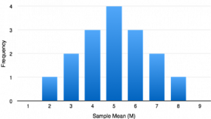
Figure 1. Distribution of sample means for n=2 from Table 1.
In our example, a population was specified (N = 4) and the sampling distribution was determined. In practice, the process actually moves the other way: you collect sample data and from these data you estimate parameters of the sampling distribution. This knowledge of the sampling distribution can be very useful. For example, knowing the degree to which means from different samples would differ from each other and from the population mean would give you a sense of how close your particular sample mean is likely to be to the population mean. This information is directly available from a sampling distribution.
We will use the NHANES dataset (National Health and Nutrition Examination Study mentioned in chapter 1) as another example; we are going to assume that the NHANES dataset is the entire population of interest, and then we will draw random samples from this population. We will have more to say in the next chapter about exactly how the generation of “random” samples works in a computer.
In this example, we know the adult population mean (168.35) and standard deviation (10.16) for height because we are assuming that the NHANES dataset is the population. Table 2 shows the statistics computed from a few samples of 50 individuals from the NHANES population.
| sampleMean | sampleSD |
|---|---|
| 167 | 9.1 |
| 171 | 8.3 |
| 170 | 10.6 |
| 166 | 9.5 |
| 168 | 9.5 |
The sample mean and standard deviation are similar but not exactly equal to the population values. Now let’s take a large number of samples of 50 individuals, compute the mean for each sample, and look at the resulting sampling distribution of means. We have to decide how many samples to take in order to do a good job of estimating the sampling distribution – in this case, we will take 5000 samples so that we are very confident in the answer. Note that simulations like this one can sometimes take a few minutes to run, and might make your computer huff and puff. The histogram in Figure 2 shows that the means estimated for each of the samples of 50 individuals vary somewhat, but that overall they are centered around the population mean. The average of the 5000 sample means (168.3463) is very close to the true population mean (168.3497).
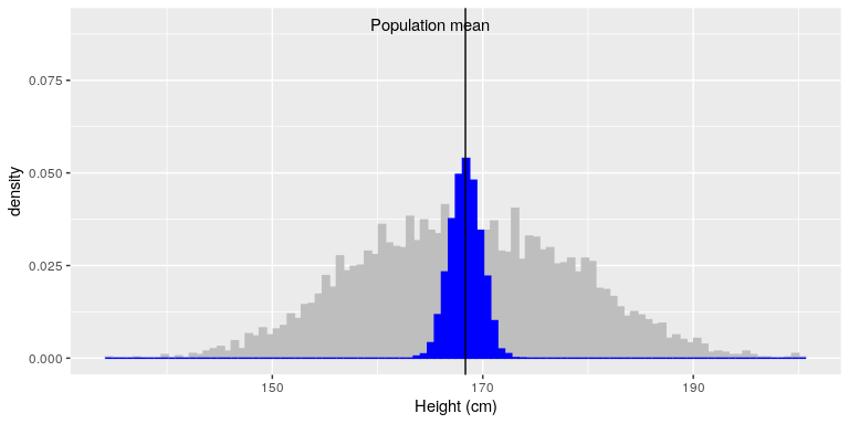
Figure 2: The blue histogram shows the sampling distribution of the mean over 5000 random samples from the NHANES dataset. The histogram for the full dataset is shown in gray for reference.
The Sampling Distribution of Sample Means
To see how we use sampling error, we will learn about a new, theoretical distribution known as the sampling distribution. In the same way that we can gather a lot of individual scores and put them together to form a distribution with a center and spread, if we were to take many samples, all of the same size, and calculate the mean of each of those, we could put those means together to form a distribution. This new distribution is, intuitively, known as the distribution of sample means. It is one example of what we call a sampling distribution, we can be formed from a set of any statistic, such as a mean, a test statistic, or a correlation coefficient (more on the latter two in Units 2 and 3). For our purposes, understanding the distribution of sample means will be enough to see how all other sampling distributions work to enable and inform our inferential analyses, so these two terms will be used interchangeably from here on out. Let’s take a deeper look at some of its characteristics.
The sampling distribution of sample means can be described by its shape, center, and spread, just like any of the other distributions we have worked with. The shape of our sampling distribution is normal: a bell-shaped curve with a single peak and two tails extending symmetrically in either direction, just like what we saw in previous chapters.
Guidelines of a Distribution of Sample Means (DSM)
In order for a distribution of sampling means (DSM) to be accurate we must draw every possible sample out of the population and plot its mean. In the first example, with our population of just four scores, it wasn’t very difficult to do this. Most populations are much larger than our simple example. In real life, to make a complete, accurate DSM we should have collected over 12 trillion samples in order to plot every sample mean possible. This is not efficient and fortunately we do not have to do it because we can estimate parameters.
If we know the mean (μ) and standard deviation (σ) of the distribution of individual scores, then we can estimate the mean and standard deviation of the distribution of sample means without having to make thousands, millions and trillions of calculations. We can follow three simple guidelines:
-
Shape
The shape of the distribution of sample means (DSM) will be normal if either one of the following two conditions are met:
We will talk more about this later, but note that with samples larger than 30, the sampling distribution of the mean is normal even if the data within each sample are not normally distributed. This is an important concept because if we want to apply the proportions and probabilities of a normal distribution then the shape of the distribution of sample means must approximate the shape. Also, not all parameters of a population follow a normal distribution and not all research questions are interested in these parameters – but with a large enough sample, even skewed population parameters can approximate the normal distribution.
2. Mean
The mean of the distribution of sampling means is the mean of the population from which the scores were sampled. Therefore, if a population has a mean μ, then the mean of the sampling distribution of the mean is also μ. The symbol μM is used to refer to the mean of the sampling distribution of the mean.
This can also be written as μx̄ to denote it as the mean of the sample means. As you can see the mean for the distribution of the sample means is exactly the same as the population mean. We would expect these values to be the same. The center of the sampling distribution of sample means – which is, itself, the mean or average of the means – is the true population mean, μ.
3. Standard Deviation
The most common measure of how much sample means differ from each other is the standard deviation of the distribution of sampling means. This standard deviation is called the standard error of the mean and it measures the expected difference between the sample mean (M) and the population mean (µ).
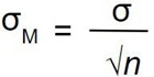
Notice that the sample size is in the standard error equation. As stated above, the sampling distribution refers to samples of a specific size. That is, all sample means must be calculated from samples of the same size n, such n = 10, n = 30, or n = 100. This sample size refers to how many people or observations are in each individual sample, not how many samples are used to form the sampling distribution. This is because the sampling distribution is a theoretical distribution, not one we will ever actually calculate or observe. Note that we have to be careful about computing standard error using the estimated standard deviation if our sample is small (less than about 30).
The formula for the standard error of the mean implies that the quality of our measurement involves two quantities: the population variability, and the size of our sample. Because the sample size is the denominator in the formula for standard error a larger sample size will yield a smaller standard error when holding the population variability constant. We have no control over the population variability, but we do have control over the sample size. Thus, if we wish to improve our sample statistics (by reducing their sampling variability) then we should use larger samples. The expected difference between sample means and population mean is closely related to the elements formula – sample size and standard deviation.
Figure 3 displays three guidelines for the distribution of sample means in graphical form.
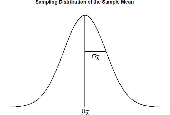
Figure 3. The sampling distribution of sample means
We can also compare this sampling distribution of the means to that of a population. Because the standard error takes the standard deviation and divides it by a number greater than 1, the value of the standard error will always be smaller than the value of the standard deviation. Also, by taking the mean of all sample means, we are automatically reducing the variability between scores. Each sample mean is a summary statistic that represents the center of that sample. A sample mean “washes out” individual high and low scores in that sample by creating the average. Further, because each sample mean (M) is an approximation of the population mean (μ), the sample means cluster more tightly around μ than individual scores. The amount of variability among sample means (σM) depends on the amount of variability among the individual scores in the population (σ) and on the size of samples (n) used to create the DSM. This is show in Figure 4 and connects back to our example in Figure 2. In other words, variability among sample means in a distribution of sample means will be reduced as sample size is increased, and/or as population variability is reduced. One way to remember this is to think about the formula we use to calculate the standard error. We calculate the standard error (σM) by dividing the standard deviation (σ) by the square root of the sample size (n).
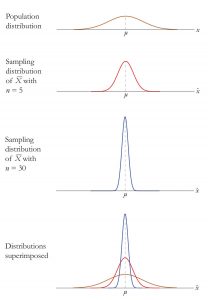
Figure 4. Distributions based on population, sample size of 5 and sample size of 30. Image credit
Two Important Axioms
Central Limit Theorem
The Central Limit Theorem:
For samples of a single size n, drawn from a population with a given mean μ and variance σ2, the sampling distribution of sample means will have a mean μ𝑋̅ = μ and variance σ2 = σ2/n. This distribution will approach normality as n increases tells us that as sample sizes get larger, the sampling distribution of the mean will become normally distributed. The last sentence of the central limit theorem states that the sampling distribution will be normal as the sample size of the samples used to create it increases. What this means is that bigger samples will create a more normal distribution, so we are better able to use the techniques we developed for normal distributions and probabilities. So how large is large enough? In general, a sampling distribution will be normal if either of two characteristics is true: 1) the population from which the samples are drawn is normally distributed or 2) the sample size is equal to or greater than 30. This second criteria is very important because it enables us to use methods developed for normal distributions even if the true population distribution is skewed.
To see the central limit theorem in action, let’s work with the variable AlcoholYear from the NHANES dataset, which is highly skewed, as shown in the left panel of Figure 5. This distribution is, for lack of a better word, funky – and definitely not normally distributed. Now let’s look at the sampling distribution of the mean for this variable. Figure 5 shows the sampling distribution for this variable, which is obtained by repeatedly drawing samples of size 50 from the NHANES dataset and taking the mean. Despite the clear non-normality of the original data, the sampling distribution is remarkably close to the normal.
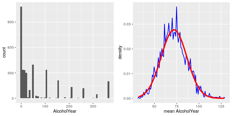
Figure 5: Left: Distribution of the variable AlcoholYear in the NHANES dataset, which reflects the number of days that the individual drank in a year. Right: The sampling distribution of the mean for AlcoholYear in the NHANES dataset, obtained by drawing repeated samples of size 50, in blue. The normal distribution with the same mean and standard deviation is shown in red.
The Central Limit Theorem is important for statistics because it allows us to safely assume that the sampling distribution of the mean will be normal in most cases. This means that we can take advantage of statistical techniques that assume a normal distribution, as we will see in the next section. It’s also important because it tells us why normal distributions are so common in the real world; any time we combine many different factors into a single number, the result is likely to be a normal distribution. For example, the height of any adult depends on a complex mixture of their genetics and experience; even if those individual contributions may not be normally distributed, when we combine them the result is a normal distribution.
Law of Large Numbers
The law of large numbers simply states that as our sample size increases, the probability that our sample mean is an accurate representation of the true population mean also increases. It is the formal mathematical way to state that larger samples are more accurate. The law of large numbers is related to the central limit theorem, specifically the formulas for variance and standard error. Notice that the sample size appears in the denominators of those formulas. A larger denominator in any fraction means that the overall value of the fraction gets smaller (i.e 1/2 = 0.50, 1/3 – 0.33, 1/4 = 0.25, and so on). Thus, larger sample sizes will create smaller standard errors. We already know that standard error is the spread of the sampling distribution and that a smaller spread creates a narrower distribution. Therefore, larger sample sizes create narrower sampling distributions, which increases the probability that a sample mean will be close to the center and decreases the probability that it will be in the tails. This is illustrated in Figures 6 and 7.
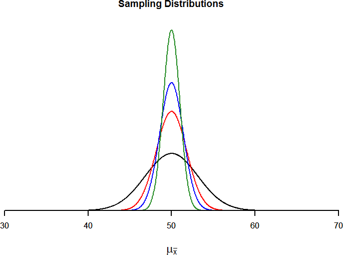
Figure 6. Sampling distributions from the same population with μ = 50 and σ = 10 but different sample sizes (n = 10, n = 30, n = 50, n = 100)
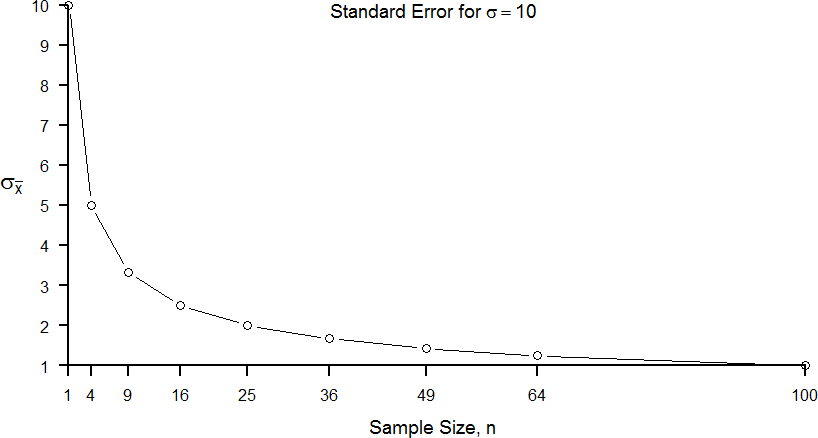
Figure 7. Relation between sample size and standard error for a constant σ = 10
Using Standard Error for Probability
We saw in chapter 7 that we can use z-scores to split up a normal distribution and calculate the proportion of the area under the curve in one of the new regions, giving us the probability of randomly selecting a z-score in that range. We can follow the exact sample process for sample means, converting them into z-scores and calculating probabilities. The only difference is that instead of dividing a raw score by the standard deviation, we divide the sample mean by the standard error.
 Remember that
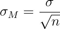
Let’s say we are drawing samples from a population with a mean of 50 and standard deviation of 10 (the same values used in Figure 6). What is the probability that we get a random sample of size 10 with a mean greater than or equal to 55? That is, for n = 10, what is the probability that ̅X ≥ 55? First, we need to convert this sample mean score into a z-score:
Z = (55-50) / 10⁄√10 = 5/3.16 = 1.58
Now we need to shade the area under the normal curve corresponding to scores greater than z = 1.58 as in Figure 8:
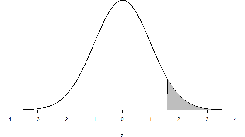
Figure 8: Area under the curve greater than z = 1.58
Now let’s do the same thing, but assume that instead of only having a sample of 10 people we took a sample of 50 people. First, we find z:
Z = (55-50)/ 10⁄√50 = 5/1.41 = 3.55
Then we shade the appropriate region of the normal distribution:
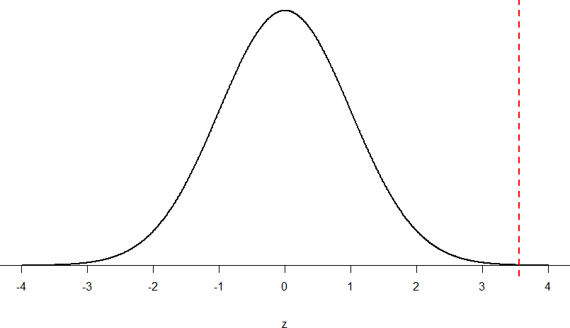
Figure 9: Area under the curve greater than z = 3.55
 Photo credit All of these pieces fit together, and the relations will always be the same: n↑ σM↓ z↑ p↓
 Let’s look at this one more way. For the same population of sample size 50 and standard deviation 10, what proportion of sample means fall between 47 and 53 if they are of sample size 10 and sample size 50?
We’ll start again with n = 10. Converting 47 and 53 into z-scores, we get z = -0.95 and z = 0.95, respectively. From our z-table, we find that the proportion between these two scores is 0.6578 (the process here is left off for the student to practice converting X to z and z to proportions). So, 65.78% of sample means of sample size 10 will fall between 47 and 53. For n = 50, our z-scores for 47 and 53 are ±2.13, which gives us a proportion of the area as 0.9668, almost 97%! Shaded regions for each of these sampling distributions is displayed in Figure 9. The sampling distributions are shown on the original scale, rather than as z-scores, so you can see the effect of the shading and how much of the body falls into the range, which is marked off with dotted line.
Figure 9. Areas between 47 and 53 for sampling distributions of n = 10 and n = 50
Sampling Distribution, Probability and Inference
We’ve seen how we can use the standard error to determine probability based on our normal curve. We can think of the standard error as how much we would naturally expect our statistic – be it a mean or some other statistic – to vary. In our formula for z based on a sample mean, the numerator (M − μ) is what we call an observed effect. That is, it is what we observe in our sample mean versus what we expected based on the population from which that sample mean was calculated.
Because the sample mean will naturally move around due to sampling error, our observed effect will also change naturally. In the context of our formula for z, then, our standard error is how much we would naturally expect the observed effect to change. Changing by a little is completely normal, but changing by a lot might indicate something is going on. This is the basis of inferential statistics and the logic behind hypothesis testing, the subject of Unit 2.
Recap
Earlier we learned that probability forms the direct link between samples and the population that they come from. This link serves as the foundation for inferential statistics.
As we learned earlier, the concept of a sampling distribution is perhaps the most basic concept in inferential statistics but it is also one of the most challenging because we have to accept hypothetical concepts and theories about how samples and normal distributions work. A few key things to remember are that the sample distribution of the means is based on sample statistics (sample means) not on individual scores. Second, the distribution of sample means is formed by statistics obtained by selecting all possible samples of a specific size from a population. The standard error of the mean is used to determine how close a sample mean is to a population mean.
When we are describing the parameters of a DSM, there are a few differences and a few similarities compared to the other distributions we have already learned about.
| measure of central tendency | measure of variability | |
| distribution of individual scores (sample) | M | S |
| distribution of individual scores (population) | µ | σ |
| distribution of sample means | M | σM |
Learning Objectives
Having read this chapter, you should be able to:
- Distinguish between a population and a sample, and between population parameters and sample statistics
- Describe the concepts of sampling error and sampling distribution
- Compute the z-score for distribution of sample means
- Compute the standard error of the mean
- Describe how the Central Limit Theorem determines the nature of the sampling distribution of the mean
- Use the distribution of sample means, z-scores, and unit normal table to determine probabilities corresponding to sample means.
We have come to the final chapter in this unit. We will now take the logic, ideas, and techniques we have developed and put them together to see how we can take a sample of data and use it to make inferences about what’s truly happening in the broader population. This is the final piece of the puzzle that we need to understand in order to have the groundwork necessary for formal hypothesis testing. Though some of the concepts in this chapter seem strange, they are all simple extensions of what we have already learned in previous chapters.
Exercises – Ch. 8
- What is a sampling distribution?
- What are the two mathematical facts that describe how sampling distributions work?
- What is the difference between a sampling distribution and a regular distribution?
- What effect does sample size have on the shape of a sampling distribution?
- What is standard error?
- For a population with a mean of 75 and a standard deviation of 12, what proportion of sample means of size n = 16 fall above 82?
- For a population with a mean of 100 and standard deviation of 16, what is the probability that a random sample of size 4 will have a mean between 110 and 130?
- Find the z-score for the following means taken from a population with mean 10 and standard deviation 2:
- ̅X = 8, n = 12
- ̅X = 8, n = 30
- ̅X = 20, n = 4
- ̅X = 20, n = 16
- As the sample size increases, what happens to the p-value associated with a given sample mean?
- For a population with a mean of 35 and standard deviation of 7, find the sample mean of size n = 20 that cuts off the top 5% of the sampling distribution.
Answers to Odd-Numbered Exercises – Ch. 8
1. The sampling distribution (or sampling distribution of the sample means) is the distribution formed by combining many sample means taken from the same population and of a single, consistent sample size.
9. As sample size increases, the p-value will decrease
