
9 Population and Community Ecology
Learning Objectives
After studying this chapter, you should be able to:
- Describe how ecologists measure population size and density
- Describe three different patterns of population distribution
- Explain the characteristics of and differences between exponential and logistic growth patterns
- Give examples of how the carrying capacity of a habitat may change
- Discuss the predator-prey cycle
- Give examples of defenses against predation and herbivory
- Describe the competitive exclusion principle
- Give examples of symbiotic relationships between species
- Describe community structure and succession
Why Study Populations and Communities?
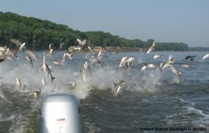
Imagine sailing down a river in a small motorboat on a weekend afternoon; the water is smooth, and you are enjoying the sunshine and cool breeze when suddenly you are hit in the head by a 20-pound silver carp (Figure 1). This is a risk now on many rivers and canal systems in Illinois and Missouri because of the presence of invasive carp species.
This fish has been farmed and eaten in China for over 1,000 years. It is one of the most important aquaculture food resources worldwide. In the United States, however, silver carp is considered a dangerous invasive species that disrupts ecological community structure to the point of threatening native species.
The effects of invasive species (such as the silver carp, kudzu vine, predatory snakehead fish, and zebra mussel) are just one aspect of what ecologists study to understand how populations interact within ecological communities, and what impact natural and human-induced disturbances have on the characteristics of communities.
Population Ecology
Populations are dynamic entities. Their size and composition fluctuate in response to numerous factors, including seasonal and yearly changes in the environment, natural disasters such as forest fires and volcanic eruptions, and competition for resources between and within species. The statistical study of populations is called demography: a set of mathematical tools designed to describe populations and investigate how they change. Many of these tools were actually designed to study human populations. For example, life tables, which detail the life expectancy of individuals within a population, were initially developed by life insurance companies to set insurance rates. In fact, while the term “demographics” is sometimes assumed to mean a study of human populations, all living populations can be studied using this approach.
Estimating Population Size
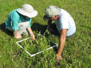
The most accurate way to determine population size is to count all of the individuals within the area. However, this method is usually not logistically or economically feasible, especially when studying large areas. Thus, scientists usually study populations by sampling a representative portion of each habitat and use this sample to make inferences about the population as a whole. The methods used to sample populations to determine their size and density are typically tailored to the characteristics of the organism being studied. For immobile organisms such as plants, or for very small and slow-moving organisms, a quadrat may be used. A quadrat is a wood, plastic, or metal square that is randomly located on the ground and used to count the number of individuals that lie within its boundaries (Figure 2). To obtain an accurate count using this method, the square must be placed at random locations within the habitat enough times to produce an accurate estimate. This counting method will provide an estimate of both population size and density. The number and size of quadrat samples depends on the type of organisms and the nature of their distribution.
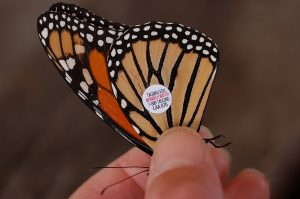
For smaller mobile organisms, such as mammals, a technique called mark and recapture is often used. This method involves humanely capturing a sample of animals, marking them in some way, and releasing them back into the environment to mix with the rest of the population (Figure 3). Then, a new sample is captured and scientists determine how many of the marked animals are in the new sample. This method assumes that the larger the population, the lower the percentage of marked organisms that will be recaptured since they will have mixed with more unmarked individuals.
The total population size can be estimated using the following equation:
[latex]\frac{number\:marked\: \times\: total\:number\:recaptured}{number\:recaptured\:with\:a\:mark} = number\:in\:population[/latex]
For example, imagine 80 field mice are captured, marked, and released back into the forest. Then in a second trapping, 100 field mice are captured, and 20 of them are marked:
[latex]\frac{80\: \times\: 100}{20} = 400[/latex]
These results give us an estimate of 400 total individuals in the original population. The true number usually will be a bit different from this because of chance errors and possible bias caused by the sampling methods.
Species Distribution
In addition to measuring density, further information about a population can be obtained by looking at the distribution of the individuals throughout their range. A species distribution pattern is the distribution of individuals within a habitat at a particular point in time—broad categories of patterns are used to describe them.
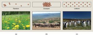
Individuals within a population can be distributed at random, in groups, or equally spaced apart (more or less). These are known as random, clumped, and uniform distribution patterns, respectively (Figure 4). Different distributions reflect important aspects of the biology of the species; they also affect the mathematical methods required to estimate population sizes.
An example of random distribution occurs with dandelion and other plants that have wind-dispersed seeds that germinate wherever they happen to fall in favorable environments. A clumped distribution, may be seen in plants that drop their seeds straight to the ground, such as oak trees; it can also be seen in animals that live in social groups (schools of fish or herds of elephants). Uniform distribution is observed in plants that secrete substances inhibiting the growth of nearby individuals (such as the release of toxic chemicals by sage plants). It is also seen in territorial animal species, such as penguins that maintain a defined territory for nesting. The territorial defensive behaviors of each individual create a regular pattern of distribution of similar-sized territories and individuals within those territories. Thus, the distribution of the individuals within a population provides more information about how they interact with each other than does a simple density measurement. Just as lower density species might have more difficulty finding a mate, solitary species with a random distribution might have a similar difficulty when compared to social species clumped together in groups.
Knowledge Check
Population Growth
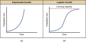
The two simplest models of population growth use deterministic equations (equations that do not account for random events) to describe the rate of change in the size of a population over time. The first of these models, exponential growth, describes theoretical populations that increase in numbers without any limits to their growth. The second model, logistic growth, introduces limits to reproductive growth that become more intense as the population size increases. Neither model adequately describes natural populations, but they provide points of comparison.
Exponential Growth
Charles Darwin, in developing his theory of natural selection, was influenced by the English clergyman Thomas Malthus. Malthus published his book in 1798 stating that populations with abundant natural resources grow very rapidly; however, they limit further growth by depleting their resources. The early pattern of accelerating population size is called exponential growth.
The best example of exponential growth in organisms is seen in bacteria. Bacteria are prokaryotes that reproduce largely by binary fission. This division takes about an hour for many bacterial species. If 1000 bacteria are placed in a large flask with an abundant supply of nutrients (so the nutrients will not become quickly depleted), the number of bacteria will have doubled from 1000 to 2000 after just an hour. In another hour, each of the 2000 bacteria will divide, producing 4000 bacteria. After the third hour, there should be 8000 bacteria in the flask. The important concept of exponential growth is that the growth rate—the number of organisms added in each reproductive generation—is itself increasing; that is, the population size is increasing at a greater and greater rate. After 24 of these cycles, the population would have increased from 1000 to more than 16 billion bacteria. When the population size, N, is plotted over time, a J-shaped growth curve is produced (Figure 5a).
Logistic Growth
Extended exponential growth is possible only when infinite natural resources are available; this is not the case in the real world. Charles Darwin recognized this fact in his description of the “struggle for existence,” which states that individuals will compete (with members of their own or other species) for limited resources. The successful ones are more likely to survive and pass on the traits that made them successful to the next generation at a greater rate (natural selection). To model the reality of limited resources, population ecologists developed the logistic growth model.
In the real world, with its limited resources, exponential growth cannot continue indefinitely. Exponential growth may occur in environments where there are few individuals and plentiful resources, but when the number of individuals gets large enough, resources will be depleted and the growth rate will slow down. Eventually, the growth rate will plateau or level off (Figure 5b). This population size, which is determined by the maximum population size that a particular environment can sustain, is called the carrying capacity, or K. In real populations, a growing population often overshoots its carrying capacity, and the death rate increases beyond the birth rate causing the population size to decline back to the carrying capacity or below it. Most populations usually fluctuate around the carrying capacity in an undulating fashion rather than existing right at a specific number.
A graph of a population undergoing logistic growth yields the S-shaped curve. It is a more realistic model of population growth than exponential growth. There are three different sections to an S-shaped curve. Initially, growth is exponential because there are few individuals and ample resources available. Then, as resources begin to become limited, the growth rate decreases. Finally, the growth rate levels off at the carrying capacity of the environment, with little change in population number over time.
Role of Intraspecific Competition
The logistic model assumes that every individual within a population will have equal access to resources and, thus, an equal chance for survival. For plants, the amount of water, sunlight, nutrients, and space to grow are the important resources, whereas in animals, important resources include food, water, shelter, nesting space, and mates.
In the real world, variation among individuals within a population means that some individuals will be better adapted to their environment than others. The resulting competition for resources among population members of the same species is termed intraspecific competition. Intraspecific competition may not affect populations that are well below their carrying capacity, as resources are plentiful and all individuals can obtain what they need. However, as population size increases, this competition intensifies. In addition, the accumulation of waste products can reduce carrying capacity in an environment.
Examples of Logistic Growth
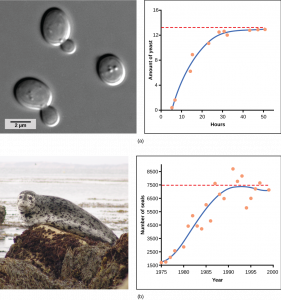
Yeast, a microscopic fungus used to make bread and alcoholic beverages, exhibits the classical S-shaped curve when grown in a test tube (Figure 6a). Its growth levels off as the population depletes the nutrients that are necessary for its growth. In the real world, however, there are variations to this idealized curve. Examples in wild populations include sheep and harbor seals (Figure 6b). In both examples, the population size exceeds the carrying capacity for short periods of time and then falls below the carrying capacity afterwards. This fluctuation in population size continues to occur as the population oscillates around its carrying capacity. Still, even with this oscillation, the logistic model is confirmed.
Community Ecology
In general, populations of one species never live in isolation from populations of other species. The interacting populations occupying a given habitat form an ecological community. The number of species occupying the same habitat and their relative abundance is known as the diversity of the community. Areas with low species diversity, such as the glaciers of Antarctica, still contain a wide variety of living organisms, whereas the diversity of tropical rainforests is so great that it cannot be accurately assessed. Scientists study ecology at the community level to understand how species interact with each other and compete for the same resources.
Predation and Herbivory
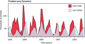
Perhaps the classical example of species interaction is the predator-prey relationship. The narrowest definition of the predator-prey interaction describes individuals of one population that kill and then consume the individuals of another population. Population sizes of predators and prey in a community are not constant over time, and they may vary in cycles that appear to be related. The most often cited example of predator-prey population dynamics is seen in the cycling of the lynx (predator) and the snowshoe hare (prey), using 100 years of trapping data from North America (Figure 7). This cycling of predator and prey population sizes has a period of approximately ten years, with the predator population lagging one to two years behind the prey population. An apparent explanation for this pattern is that as the hare numbers increase, there is more food available for the lynx, allowing the lynx population to increase as well. When the lynx population grows to a threshold level, however, they kill so many hares that hare numbers begin to decline, followed by a decline in the lynx population because of scarcity of food. When the lynx population is low, the hare population size begins to increase due, in part, to low predation pressure, starting the cycle anew.
Defense Mechanisms against Predation and Herbivory
Predation and predator avoidance are strong selective agents. Any inheritable trait that allows an individual of a prey population to better evade its predators will be represented in greater numbers in later generations. Likewise, traits that allow a predator to more efficiently locate and capture its prey will lead to a greater number of offspring and an increase in the commonness of the trait within the population. Such ecological relationships between specific populations lead to adaptations that are driven by reciprocal evolutionary responses in those populations. Species have evolved numerous mechanisms to escape predation and herbivory (the consumption of plants for food). Defenses may be mechanical, chemical, physical, or behavioral.
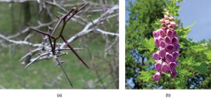
Mechanical defenses, such as the presence of armor in animals or thorns in plants, discourage predation and herbivory by discouraging physical contact (Figure 8a). Many plant species produce chemical defenses in the form of compounds that serve no function for the plant except that they are toxic to animals and discourage consumption. For example, the foxglove produces several compounds, including digitalis, that are extremely toxic when eaten (Figure 8b). Biomedical scientists have extracted the chemical produced by foxglove to use as a heart medication, which has saved lives for many decades. Animals may also produce chemical defenses or obtain them from plants and store them to prevent predation.
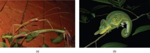
Many species use their body shape and coloration to avoid being detected by predators. The tropical walking stick is an insect with the coloration and body shape of a twig, which makes it very hard to see when it is stationary against a background of real twigs (Figure 9a). In another example, the chameleon can change its color to match its surroundings (Figure 9b).
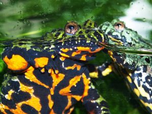
Some species use coloration as a way of warning predators that they are distasteful or poisonous. For example, the monarch butterfly caterpillar sequesters poisons from its food (milkweed plants) to make itself poisonous or distasteful to potential predators. The caterpillar is bright yellow and black to advertise its toxicity. The caterpillar is also able to pass the sequestered toxins on to the adult monarch, which is also dramatically colored black and red as a warning to potential predators. Fire-bellied toads produce toxins that make them distasteful to their potential predators. They have bright red or orange coloration on their bellies, which they display to a potential predator to advertise their poisonous nature and discourage an attack. These are only two examples of warning coloration, which is a relatively common adaptation. Warning coloration only works if a predator uses eyesight to locate prey and can learn—a naïve predator must experience the negative consequences of eating one before it will avoid other similarly colored individuals (Figure 10).
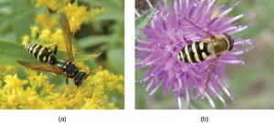
While some predators learn to avoid eating certain potential prey because of their coloration, other species have evolved mechanisms to mimic this coloration to avoid being eaten, even though they themselves may not be unpleasant to eat or contain toxic chemicals. In some cases of mimicry, a harmless species imitates the warning coloration of a harmful species. Assuming they share the same predators, this coloration then protects the harmless ones. Many insect species mimic the coloration of wasps, which are stinging, venomous insects, thereby discouraging predation (Figure 11).
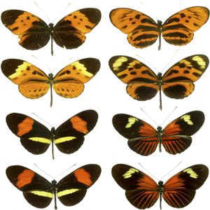
In other cases of mimicry, multiple species share the same warning coloration, but all of them actually have defenses. The commonness of the signal improves the compliance of all the potential predators. Figure 12 shows a variety of foul-tasting butterflies with similar coloration.
Competitive Exclusion Principle
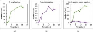
Resources are often limited within a habitat and multiple species may compete to obtain them. Ecologists have come to understand that all species have an ecological niche. A niche is the unique set of resources used by a species, which includes its interactions with other species. The competitive exclusion principle states that two species cannot occupy the same niche in a habitat: in other words, different species cannot coexist in a community if they are competing for all the same resources. This principle works because if there is an overlap in resource use and therefore competition between two species, then traits that lessen reliance on the shared resource will be selected for leading to evolution that reduces the overlap. If either species is unable to evolve to reduce competition, then the species that most efficiently exploits the resource will drive the other species to extinction. An experimental example of this principle is shown in Figure 13 with two protozoan species: Paramecium aurelia and Paramecium caudatum. When grown individually in the laboratory, they both thrive. But when they are placed together in the same test tube (habitat), P. aurelia out-competes P. caudatum for food, leading to the latter’s eventual extinction.
Symbiosis
Symbiotic relationships, also known as symbioses, are close, long-term interactions between individuals of different species. Symbioses may be commensal, in which one species benefits while the other is neither harmed nor benefited; mutualistic, in which both species benefit; or parasitic, in which the interaction harms one species and benefits the other.
Commensalism
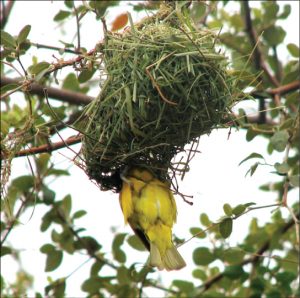
A commensal relationship occurs when one species benefits from a close prolonged interaction, while the other neither benefits nor is harmed. Birds nesting in trees provide an example of a commensal relationship (Figure 14). The tree is not harmed by the presence of the nest among its branches. The nests are light and produce little strain on the structural integrity of the branch, and most of the leaves, which the tree uses to get energy by photosynthesis, are above the nest so they are unaffected. The bird, on the other hand, benefits greatly. If the bird had to nest in the open, its eggs and young would be vulnerable to predators. Many potential commensal relationships are difficult to identify because it is difficult to prove that one partner does not derive at least some benefit from the presence of the other.
Mutualism
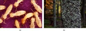
A second type of symbiotic relationship is called mutualism, in which two species benefit from their interaction. For example, termites have a mutualistic relationship with single-celled protists that live in the insect’s gut (Figure 15a). The termite benefits from the ability of the protists to digest cellulose. However, the protists are able to digest cellulose only because of the presence of symbiotic bacteria within their cells that produce the cellulase enzyme. The termite itself cannot do this: without the protozoa, it would not be able to obtain energy from its food (cellulose from the wood it chews and eats). The protozoa benefit by having a protective environment and a constant supply of food from the wood chewing actions of the termite. Lichens are a mutualistic relationship between a fungus and photosynthetic algae or cyanobacteria (Figure 15b). The glucose produced by the algae provides nourishment for both organisms, whereas the physical structure of the lichen protects the algae from the elements and makes certain nutrients in the atmosphere more available to the algae. The algae of lichens can live independently given the right environment, but many of the fungal partners are unable to live on their own.
Parasitism
A parasite is an organism that feeds off another without immediately killing the organism it is feeding on. In this relationship, the parasite benefits, but the organism being fed upon, the host, is harmed. The host is usually weakened by the parasite as it siphons resources the host would normally use to maintain itself. Parasites may kill their hosts, but there is usually selection to slow down this process to allow the parasite time to complete its reproductive cycle before it or its offspring are able to spread to another host.
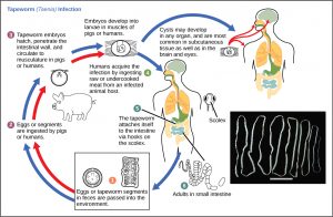
The reproductive cycles of parasites are often very complex, sometimes requiring more than one host species. A tapeworm causes disease in humans when contaminated, undercooked meat such as pork, fish, or beef is consumed (Figure 16). The tapeworm can live inside the intestine of the host for several years, benefiting from the host’s food, and it may grow to be over 50 feet long by adding segments. The parasite moves from one host species to a second host species in order to complete its life cycle. Plasmodium falciparum is another parasite: the protists that cause malaria, a significant disease in many parts of the world. Living inside human liver and red blood cells, the organism reproduces asexually in the human host and then sexually in the gut of blood-feeding mosquitoes to complete its life cycle. Thus malaria is spread from human to mosquito and back to human, one of many arthropod-borne infectious diseases of humans.
Knowledge Check
Characteristics of Communities
Communities are complex systems that can be characterized by their structure (the number and size of populations and their interactions) and dynamics (how the members and their interactions change over time). Understanding community structure and dynamics allows us to minimize impacts on ecosystems and manage ecological communities we benefit from.
Biodiversity
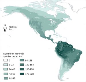
Ecologists have extensively studied one of the fundamental characteristics of communities: biodiversity. One measure of biodiversity used by ecologists is the number of different species in a particular area and their relative abundance. The area in question could be a habitat, a biome, or the entire biosphere. Species richness is the term used to describe the number of species living in a habitat or other unit. Species richness varies across the globe (Figure 17). Ecologists have struggled to understand the determinants of biodiversity. Species richness is related to latitude: the greatest species richness occurs near the equator and the lowest richness occurs near the poles. Other factors influence species richness as well. Island biogeography attempts to explain the great species richness found in isolated islands, and has found relationships between species richness, island size, and distance from the mainland.
Relative species abundance is the number individuals in a species relative to the total number of individuals in all species within a system. Foundation species, described below, often have the highest relative abundance of species.
Foundation Species
Foundation species are considered the “base” or “bedrock” of a community, having the greatest influence on its overall structure. They are often primary producers, and they are typically an abundant organism. For example, kelp, a species of brown algae, is a foundation species that forms the basis of the kelp forests off the coast of California.
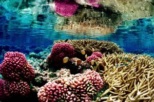
Foundation species may physically modify the environment to produce and maintain habitats that benefit the other organisms that use them. Examples include the kelp described above or tree species found in a forest. The photosynthetic corals of the coral reef also provide structure by physically modifying the environment (Figure 18). The exoskeletons of living and dead coral make up most of the reef structure, which protects many other species from waves and ocean currents.
Keystone Species
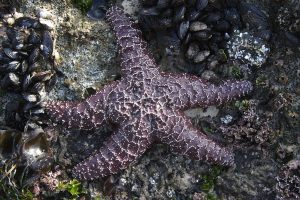
A keystone species is one whose presence has inordinate influence in maintaining the prevalence of various species in an ecosystem, the ecological community’s structure, and sometimes its biodiversity. Pisaster ochraceus, the intertidal sea star, is a keystone species in the northwestern portion of the United States (Figure 19). Studies have shown that when this organism is removed from communities, mussel populations (their natural prey) increase, which completely alters the species composition and reduces biodiversity. Another keystone species is the banded tetra, a fish in tropical streams, which supplies nearly all of the phosphorus, a necessary inorganic nutrient, to the rest of the community. The banded tetra feeds largely on insects from the terrestrial ecosystem and then excretes phosphorus into the aquatic ecosystem. The relationships between populations in the community, and possibly the biodiversity, would change dramatically if these fish were to become extinct.
Invasive Species
Invasive species are non-native organisms that, when introduced to an area out of its native range, alter the community they invade. In the United States, invasive species like the purple loosestrife (Lythrum salicaria) and the zebra mussel (Dreissena polymorpha) have altered aquatic ecosystems, and some forests are threatened by the spread of common buckthorn (Rhamnus cathartica) and garlic mustard (Alliaria petiolata). Some well-known invasive animals include the emerald ash borer (Agrilus planipennis) and the European starling (Sturnus vulgaris). Whether enjoying a forest hike, taking a summer boat trip, or simply walking down an urban street, you have likely encountered an invasive species.
One of the many recent proliferations of an invasive species concerns the Asian carp in the United States. Several species of Asian carp were introduced to the United States in the 1970s by fisheries (commercial catfish ponds) and by sewage treatment facilities that used the fish’s excellent filter feeding abilities to clean their ponds of excess plankton. Some of the fish escaped, and by the 1980s they had colonized many waterways of the Mississippi River basin, including the Illinois and Missouri Rivers.
Voracious feeders and rapid reproducers, Asian carp may outcompete native species for food and could lead to their extinction. One species, the grass carp, feeds on phytoplankton and aquatic plants. It competes with native species for these resources and alters nursery habitats for other fish by removing aquatic plants. Another species, the silver carp, competes with native fish that feed on zooplankton. In some parts of the Illinois River, Asian carp constitute 95 percent of the community’s biomass. Although edible, the fish is bony and not desired in the United States. Moreover, their presence now threatens the native fish and fisheries of the Great Lakes, which are important to local economies and recreational anglers. Asian carp have even injured humans. The fish, frightened by the sound of approaching motorboats, thrust themselves into the air, often landing in the boat or directly hitting boaters.
The Great Lakes and their prized salmon and lake trout fisheries are being threatened by Asian carp species. The carp are not yet present in the Great Lakes, and attempts are being made to prevent its access to the lakes through the Chicago Ship and Sanitary Canal, which is the only connection between the Mississippi River and Great Lakes basins. To prevent the Asian carp from leaving the canal, a series of electric barriers have been used to discourage their migration; however, the threat is significant enough that several states and Canada have sued to have the Chicago channel permanently cut off from Lake Michigan. Local and national politicians have weighed in on how to solve the problem. In general, governments have been ineffective in preventing or slowing the introduction of invasive species.
The issues associated with Asian carp show how population and community ecology, fisheries management, and politics intersect on issues of vital importance to the human food supply and economy. Socio-political issues like the Asian carp make extensive use of the sciences of population ecology, the study of members of a particular species occupying a habitat; and community ecology, the study of the interaction of all species within a habitat.
Community Dynamics
Community dynamics are the changes in community structure and composition over time, often following environmental disturbances such as volcanoes, earthquakes, storms, fires, and climate change. Communities with a relatively constant number of species are said to be at equilibrium. The equilibrium is dynamic with species identities and relationships changing over time, but maintaining relatively constant numbers. Following a disturbance, the community may or may not return to the equilibrium state.
Succession describes the sequential appearance and disappearance of species in a community over time after a severe disturbance. In primary succession, newly exposed or newly formed rock is colonized by living organisms; in secondary succession, a part of an ecosystem is disturbed and remnants of the previous community remain. In both cases, there is a sequential change in species until a more or less permanent community develops.
Primary Succession and Pioneer Species
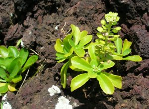
Primary succession occurs when new land is formed, for example, following the eruption of volcanoes, such as those on the Big Island of Hawaii. As lava flows into the ocean, new land is continually being formed. On the Big Island, approximately 32 acres of land is added to it its size each year. Weathering and other natural forces break down the rock enough for the establishment of hearty species such as lichens and some plants, known as pioneer species (Figure 20). These species help to further break down the mineral-rich lava into soil where other, less hardy but more competitive species, such as grasses, shrubs, and trees, will grow and eventually replace the pioneer species. Over time the area will reach an equilibrium state, with a set of organisms quite different from the pioneer species.
Secondary Succession
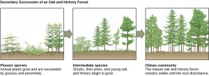
A classic example of secondary succession occurs in oak and hickory forests cleared by wildfire (Figure 21). Wildfires will burn most vegetation, and unless the animals can flee the area, they are killed. Their nutrients, however, are returned to the ground in the form of ash. Thus, although the community has been dramatically altered, there is a soil ecosystem present that provides a foundation for rapid recolonization.
Before the fire, the vegetation was dominated by tall trees with access to the major plant energy resource: sunlight. Their height gave them access to sunlight while also shading the ground and other low-lying species. After the fire, though, these trees are no longer dominant. Thus, the first plants to grow back are usually annual plants followed within a few years by quickly growing and spreading grasses and other pioneer species. Due, at least in part, to changes in the environment brought on by the growth of grasses and small non-woody plants, over many years, shrubs emerge along with small pine, oak, and hickory trees. These organisms are called intermediate species. Eventually, over 150 years, the forest will reach its equilibrium point and resemble the community before the fire. This equilibrium state is referred to as the climax community, which will remain until the next disturbance. The climax community is typically characteristic of a given climate and geology. Although the community in equilibrium looks the same once it is attained, the equilibrium is a dynamic one with constant changes in abundance and sometimes species identities. The return of a natural ecosystem after agricultural activities is also a well-documented secondary succession process.
Knowledge Check
Attribution
“Population Demographics and Dynamics” in OpenStax Concepts of Biology, modified by Sean Whitcomb. License: CC BY
“Population Growth and Regulation” in OpenStax Concepts of Biology, modified by Sean Whitcomb. License: CC BY
“Community Ecology” in OpenStax Concepts of Biology, modified by Sean Whitcomb. License: CC BY
Media Attributions
- asian-carp-usgs © USGS is licensed under a Public Domain license
- Quadrat © FWC Fish and Wildlife Research Institute is licensed under a CC BY-NC-ND (Attribution NonCommercial NoDerivatives) license
- Monarch_Butterfly_Danaus_plexippus_Tagged_Closeup_3008px © Derek Ramsey is licensed under a CC BY-SA (Attribution ShareAlike) license
- Species_distribution © Rosendahl; Rebecca Wood; Ben Tubby adapted by OpenStax is licensed under a CC BY (Attribution) license
- Exponential_logistic_growth © OpenStax is licensed under a CC BY (Attribution) license
- Logistic_growth © OpenStax is licensed under a CC BY (Attribution) license
- Hare_lynx_population © CFCF is licensed under a CC BY (Attribution) license
- Predation_defense © Huw Williams; Philip Jägenstedt adapted by OpenStax is licensed under a CC BY (Attribution) license
- Camouflage © Linda Tanner; Frank Vassen adapted by OpenStax is licensed under a CC BY (Attribution) license
- Fire-bellied toad © Robert Verzo adapted by OpenStax is licensed under a CC BY (Attribution) license
- Mimicry_wasp_hoverfly © Tom Ings adapted by OpenStax is licensed under a CC BY (Attribution) license
- Mimicry_butterflies © Joron M, Papa R, Beltrán M, Chamberlain N, Mavárez J, et al. is licensed under a CC BY (Attribution) license
- Paramecium_graphs © OpenStax is licensed under a CC BY (Attribution) license
- Bird_nest © Hanay is licensed under a CC BY (Attribution) license
- Mutualism © Scott Bauer, USDA; Cory Zanker is licensed under a CC BY (Attribution) license
- Tapeworm_life_cycle © CDC adapted by OpenStax is licensed under a Public Domain license
- Mammal species richness map © NASA; CIESIN; Columbia University adapted by OpenStax is licensed under a CC BY (Attribution) license
- Coral © Jim E. Maragos, U.S. FWS is licensed under a Public Domain license
- Starfish © Jerry Kirkhart is licensed under a CC BY (Attribution) license
- Succulents on volcanic soil © Forest and Kim Starr is licensed under a CC BY (Attribution) license
- Secondary_succession © OpenStax is licensed under a CC BY (Attribution) license

_(2132256087).jpg)