Chapter 9 Hypothesis testing

Alisa Beyer

9 Chapter 9 Hypothesis testing

Foundation for hypothesis testing

The first unit was designed to prepare you for hypothesis testing explaining descriptive statistics, standardized scores, probability, and distributions. In the first chapter, we discussed the three major goals of statistics:

Describe: connects to unit 1 with descriptive statistics and graphing
Decide: connects to unit 1 knowing your data and hypothesis testing (this chapter)
Predict: connects to hypothesis testing and unit 3

The remaining chapters will cover many different kinds of hypothesis tests connected to different inferential statistics. Needless to say, hypothesis testing is the central topic of this course. This lesson is important, but that does not mean the same thing as being difficult. There is a lot of new language we will learn about when conducting a hypothesis test. Some of the components of a hypothesis test are the topics we are already familiar with:

Test statistics
Probability
Distribution of sample means (DSM)

Hypothesis Testing

Hypothesis testing is an inferential procedure that uses data from a sample to draw a general conclusion about a population. It is a formal approach and a statistical method that uses sample data to evaluate hypotheses about a population. When interpreting a research question and statistical results, a natural question arises as to whether the finding could have occurred by chance. Hypothesis testing is a statistical procedure for testing whether chance (random events) is a reasonable explanation of an experimental finding. Once you have mastered the material in this lesson you will be used to solving hypothesis testing problems and the rest of the course will seem much easier. In this chapter, we will introduce the ideas behind the use of statistics to make decisions – in particular, decisions about whether a particular hypothesis is supported by the data.

Logic and Purpose of Hypothesis Testing

History of hypothesis testing

The statistician Ronald Fisher explained the concept of hypothesis testing with a story of a lady tasting tea. Fisher was a statistician from London and is noted as the first person to formalize the process of hypothesis testing. His elegantly simple “Lady Tasting Tea” experiment demonstrated the logic of the hypothesis test.

blonde drinking a cup of tea

Figure 1. A depiction of the lady tasting tea Photo Credit

Fisher would often have afternoon tea during his studies. He usually took tea with a woman who claimed to be a tea expert. In particular, she told Fisher that she could tell which was poured first in the teacup, the milk or the tea, simply by tasting the cup. Fisher, being a scientist, decided to put this rather bizarre claim to the test. The lady accepted his challenge. Fisher brought her 8 cups of tea in succession; 4 cups would be prepared with the milk added first, and 4 with the tea added first. The cups would be presented in a random order unknown to the lady.

The lady would take a sip of each cup as it was presented and report which ingredient she believed was poured first. Using the laws of probability, Fisher determined the chances of her guessing all 8 cups correctly was 1/70, or about 1.4%. In other words, if the lady was indeed guessing there was a 1.4% chance of her getting all 8 cups correct. On the day of the experiment, Fisher had 8 cups prepared just as he had requested. The lady drank each cup and made her decisions for each one.

After the experiment, it was revealed that the lady got all 8 cups correct! Remember, had she been truly guessing, the chance of getting this result was 1.4%. Since this probability was so low, Fisher instead concluded that the lady could indeed differentiate between the milk or the tea being poured first. Fisher’s original hypothesis that she was just guessing was demonstrated to be false and was therefore rejected. The alternative hypothesis, that the lady could truly tell the cups apart, was then accepted as true.

This story demonstrates many components of hypothesis testing in a very simple way. For example, Fisher started with a hypothesis that the lady was guessing. He then determined that if she was indeed guessing, the probability of guessing all 8 right was very small, just 1.4%. Since that probability was so tiny, when she did get all 8 cups right, Fisher determined it was extremely unlikely she was guessing. A more reasonable conclusion was that the lady had the skill to tell the cups apart.

In hypothesis testing, we will always set up a particular hypothesis that we want to demonstrate to be true. We then use probability to determine the likelihood of our hypothesis is correct. If it appears our original hypothesis was wrong, we reject it and accept the alternative hypothesis. The alternative hypothesis is usually the opposite of our original hypothesis. In Fisher’s case (box featured above), his original hypothesis was that the lady was guessing. His alternative hypothesis was the lady was not guessing.

Let’s consider this with a James Bond twist. James Bond insisted that martinis should be shaken rather than stirred. Let’s consider a hypothetical experiment to determine whether Mr. Bond can tell the difference between a shaken and a stirred martini. Suppose we gave Mr. Bond a series of 16 taste tests. In each test, we flipped a fair coin to determine whether to stir or shake the martini (i.e., random assignment). Then we presented the martini to Mr. Bond and asked him to decide whether it was shaken or stirred. Let’s say Mr. Bond was correct on 13 of the 16 taste tests. Does this prove that Mr. Bond has at least some ability to tell whether the martini was shaken or stirred?

This result does not prove that he does; it could be he was just lucky and guessed right 13 out of 16 times. But how plausible is the explanation that he was just lucky? To assess its plausibility, we determine the probability that someone who was just guessing would be correct 13/16 times or more. This probability can be computed to be 0.0106. This is a pretty low probability, and therefore someone would have to be very lucky to be correct 13 or more times out of 16 if they were just guessing. A low probability gives us more confidence there is evidence Bond can tell whether the drink was shaken or stirred. There is also still a chance that Mr. Bond was very lucky (more on this later!). The hypothesis that he was guessing is not proven false, but considerable doubt is cast on it. Therefore, there is strong evidence that Mr. Bond can tell whether a drink was shaken or stirred.

You may notice some patterns here:

We have 2 hypotheses: the original (researcher prediction) and the alternative
We collect data
We determine how likely or unlikely the original hypothesis is to occur based on probability.
We determine if we have enough evidence to support the original hypothesis and draw conclusions.

Hypothesis Testing Terminology

Now let’s begin with some specific terminology:

Null hypothesis: In general, the null hypothesis, written H₀ (“H-naught”), is the idea that nothing is going on: there is no effect of our treatment, no relation between our variables, and no difference in our sample mean from what we expected about the population mean. The null hypothesis indicates that an apparent effect is due to chance. This is always our baseline starting assumption, and it is what we (typically) seek to reject. For mathematical notation, one uses =).

Alternative hypothesis: If the null hypothesis is rejected, then we will need some other explanation, which we call the alternative hypothesis, H_A or H₁. The alternative hypothesis is simply the reverse of the null hypothesis. Thus, our alternative hypothesis is the mathematical way of stating our research question. In general, the alternative hypothesis (also called the research hypothesis)is there is an effect of treatment, the relation between variables, or differences in a sample mean compared to a population mean. The alternative hypothesis essentially shows evidence the findings are not due to chance. It is also called the research hypothesis as this is the most common outcome a researcher is looking for: evidence of change, differences, or relationships. There are three options for setting up the alternative hypothesis, depending on where we expect the difference to lie. The alternative hypothesis always involves some kind of inequality (≠not equal, >, or <).

If we expect a specific direction of change/differences/relationships, which we call a directional hypothesis, then our alternative hypothesis takes the form based on the research question itself. One would expect a decrease in depression from taking an anti-depressant as a specific directional hypothesis. Or the direction could be larger, where for example, one might expect an increase in exam scores after completing a student success exam preparation module. The directional hypothesis (2 directions) makes up 2 of the 3 alternative hypothesis options. The other alternative is to state there are differences/changes, or a relationship but not predict the direction. We use a non-directional alternative hypothesis (typically see ≠ for mathematical notation).

Probability value (p-value): the probability of a certain outcome assuming a certain state of the world. In statistics, it is conventional to refer to possible states of the world as hypotheses since they are hypothesized states of the world. Using this terminology, the probability value is the probability of an outcome given the hypothesis. It is not the probability of the hypothesis given the outcome. It is very important to understand precisely what the probability values mean. In the James Bond example, the computed probability of 0.0106 is the probability he would be correct on 13 or more taste tests (out of 16) if he were just guessing. It is easy to mistake this probability of 0.0106 as the probability he cannot tell the difference. This is not at all what it means. The probability of 0.0106 is the probability of a certain outcome (13 or more out of 16) assuming a certain state of the world (James Bond was only guessing).

A low probability value casts doubt on the null hypothesis. How low must the probability value be in order to conclude that the null hypothesis is false? Although there is clearly no right or wrong answer to this question, it is conventional to conclude the null hypothesis is false if the probability value is less than 0.05 (p < .05). More conservative researchers conclude the null hypothesis is false only if the probability value is less than 0.01 (p<.01). When a researcher concludes that the null hypothesis is false, the researcher is said to have rejected the null hypothesis. The probability value below which the null hypothesis is rejected is called the α level or simply α (“alpha”). It is also called the significance level. If α is not explicitly specified, assume that α = 0.05.

Decision-making is part of the process and we have some language that goes along with that. Importantly, null hypothesis testing operates under the assumption that the null hypothesis is true unless the evidence shows otherwise. We (typically) seek to reject the null hypothesis, giving us evidence to support the alternative hypothesis. If the probability of the outcome given the hypothesis is sufficiently low, we have evidence that the null hypothesis is false. Note that all probability calculations for all hypothesis tests center on the null hypothesis. In the James Bond example, the null hypothesis is that he cannot tell the difference between shaken and stirred martinis. The probability value is low that one is able to identify 13 of 16 martinis as shaken or stirred (0.0106), thus providing evidence that he can tell the difference. Note that we have not computed the probability that he can tell the difference.

The specific type of hypothesis testing reviewed is specifically known as null hypothesis statistical testing (NHST). We can break the process of null hypothesis testing down into a number of steps a researcher would use.

Formulate a hypothesis that embodies our prediction (before seeing the data)
Specify null and alternative hypotheses
Collect some data relevant to the hypothesis
Compute a test statistic
Identify the criteria probability (or compute the probability of the observed value of that statistic) assuming that the null hypothesis is true
Drawing conclusions. Assess the “statistical significance” of the result

The Court Case Analogy

In a criminal trial, the defendant is presumed innocent until proven guilty. Similarly, in null hypothesis testing:

The “null hypothesis” is like the presumption of innocence
It assumes there is no significant effect or relationship (the “zero” hypothesis)
This null must be disproven with strong evidence

The prosecution must provide compelling evidence to prove guilt. In statistical terms:

Researchers must collect data (evidence) to support their alternative hypothesis
The alternative hypothesis is similar to the prosecution’s claim of guilt

Courts require proof “beyond a reasonable doubt” to convict. In statistics:

We use a significance level (usually 0.05 or 5%) as our standard
This is like saying we need to be 95% certain before we “convict” (reject the null)

A trial can end in two ways, much like hypothesis testing:

Guilty verdict = Reject the null hypothesis
- Strong evidence against innocence/null hypothesis
- Accept the alternative hypothesis
- There still is a possibility for an error in our decision (more on this later in the chapter)
Not guilty verdict = Fail to reject the null hypothesis
- Insufficient evidence to prove guilt/alternative hypothesis
- We don’t prove innocence, we just lack evidence to reject it
- There still is a possibility for an error in our decision (more on this later in the chapter)

Steps in hypothesis testing

Let’s consider another example as we set up some more formal steps for hypothesis testing that we will use throughout the semester. An experiment was done to determine whether physicians spend less time with obese patients, we will refer to the study as Physicians’ Reactions. Physicians were sampled randomly and each was shown a chart of a patient complaining of a migraine headache. They were then asked to estimate how long they would spend with the patient. The charts were identical except that for half the charts, the patient was obese and for the other half, the patient was of average weight. The chart a particular physician viewed was determined randomly. Thirty-three physicians viewed charts of average-weight patients and 38 physicians viewed charts of obese patients.

Identify some key aspects of the study design: it is an experiment with 2 levels or groups in the independent variable (IV) and random assignment was used to place physicians into only 1 level/group/condition. IV has 2 categories and is classified as a nominal scale of measurement. The outcome variable being examined is the dependent variable (DV), which is estimated minutes to examine the medical chart. Minutes can be classified as a ratio scale of measurement.

Step 1: Formulate a hypothesis of interest

The researchers hypothesized that physicians spend less time with obese patients. The researchers hypothesis derived from an identified population. In creating a research hypothesis, we also have to decide whether we want to test a directional or non-directional hypotheses. Researchers typically will select a non-directional hypothesis for a more conservative approach, particularly when the outcome is unknown (more about why this is later).

Step 2: Specify the null and alternative hypotheses

Can you set up the null and alternative hypotheses for the Physician’s Reaction Experiment?

In the Physicians’ Reactions example, the null hypothesis is that in the population of physicians, the mean time expected to be spent with obese patients is equal to the mean time expected to be spent with average-weight patients. This null hypothesis can be written as: H0:μ_obese – μ_average = 0.

In the Physicians’ Reactions example, the alternative hypothesis is that in the population of physicians, the mean time expected to be spent with obese patients is equal to the mean time expected to be spent with average-weight patients. This null hypothesis can be written as: H1: μ_obese – μ_average ≠ 0. Again, it is more common to take a non-directional approach. However, if there was previous research or evidence for physicians spending less time with obese patients, the alternative hypothesis could be written as: H1: μ_obese – μ_average < 0.

A reminder that in setting up hypotheses, you will see parameters (μ for mean) used in hypotheses as we are interested in understanding the population, not just our sample (making an inference from the sample to a population for inferential statistics).

Step 3: Determine the alpha level.

For this course, alpha will be given to you as .05 or .01. Researchers will decide on alpha and then determine the associated test statistic based from the sample. Researchers in the Physician Reaction study might set the alpha at .05 and identify the test statistics associated with the .05 for the sample size. Researchers might take extra precautions to be more confident in their findings (more on this later).

Step 4: Collect some data

For this course, the data will be given to you. Researchers collect the data and then start to summarize it using descriptive statistics. The mean time physicians reported that they would spend with obese patients was 24.7 minutes as compared to a mean of 31.4 minutes for normal-weight patients.

Step 5: Compute a test statistic

We next want to use the data to compute a statistic that will ultimately let us decide whether the null hypothesis is rejected or not. We can think of the test statistic as providing a measure of the size of the effect compared to the variability in the data. In general, this test statistic will have a probability distribution associated with it, because that allows us to determine how likely our observed value of the statistic is under the null hypothesis.

To assess the plausibility of the hypothesis that the difference in mean times is due to chance, we compute the probability of getting a difference as large or larger than the observed difference (31.4 – 24.7 = 6.7 minutes) if the difference were, in fact, due solely to chance.

Step 6: Determine the probability of the observed result under the null hypothesis

Using methods presented in later chapters, this probability associated with the observed differences between the two groups for the Physician’s Reaction was computed to be 0.0057. Since this is such a low probability, we have confidence that the difference in times is due to the patient’s weight (obese or not) (and is not due to chance). We can then reject the null hypothesis (there are no differences or differences seen are due to chance).

Keep in mind that the null hypothesis is typically the opposite of the researcher’s hypothesis. In the Physicians’ Reactions study, the researchers hypothesized that physicians would expect to spend less time with obese patients. The null hypothesis that the two types of patients are treated identically as part of the researcher’s control of other variables. If the null hypothesis were true, a difference as large or larger than the sample difference of 6.7 minutes would be very unlikely to occur. Therefore, the researchers rejected the null hypothesis of no difference and concluded that in the population, physicians intend to spend less time with obese patients.

This is the step where NHST starts to violate our intuition. Rather than determining the likelihood that the null hypothesis is true given the data, we instead determine the likelihood under the null hypothesis of observing a statistic at least as extreme as one that we have observed — because we started out by assuming that the null hypothesis is true (show me the evidence)! To do this, we need to know the expected probability distribution for the statistic under the null hypothesis, so that we can ask how likely the result would be under that distribution. This will be determined from a table we use for reference or calculated in a statistical analysis program. Note that when I say “how likely the result would be”, what I really mean is “how likely the observed result or one more extreme would be”. We need to add this caveat as we are trying to determine how weird our result would be if the null hypothesis were true, and any result that is more extreme will be even more weird, so we want to count all of those weirder possibilities when we compute the probability of our result under the null hypothesis.

Step 7: Assess the “statistical significance” of the result. Draw conclusions.

The next step is to determine whether the p-value that results from the previous step is small enough that we are willing to reject the null hypothesis and conclude instead that the alternative is true. In the Physicians Reactions study, the probability value is 0.0057. Therefore, the effect of obesity is statistically significant and the null hypothesis that obesity makes no difference is rejected. It is very important to keep in mind that statistical significance means only that the null hypothesis of exactly no effect is rejected; it does not mean that the effect is important, which is what “significant” usually means. When an effect is significant, you can have confidence the effect is not exactly zero. Finding that an effect is significant does not tell you about how large or important the effect is.

How much evidence do we require and what considerations are needed to better understand the significance of the findings? This is one of the most controversial questions in statistics, in part because it requires a subjective judgment – there is no “correct” answer.

**Let’s review some considerations for Null hypothesis statistical testing (NHST)!**

Null hypothesis statistical testing (NHST) is commonly used in many fields. If you pick up almost any scientific or biomedical research publication, you will see NHST being used to test hypotheses. Thus, learning how to use and interpret the results from hypothesis testing is essential to understand the results from many fields of research.

It is also important for you to know, however, that NHST is flawed, and that many statisticians and researchers think that it has been the cause of serious problems in science, which we will discuss in further in this unit. NHST is also widely misunderstood, largely because it violates our intuitions about how statistical hypothesis testing should work.

Let’s look at an example to see this.

There is great interest in the use of body-worn cameras by police officers, which are thought to reduce the use of force and improve officer behavior. However, in order to establish this we need experimental evidence, and it has become increasingly common for governments to use randomized controlled trials to test such ideas. A randomized controlled trial of the effectiveness of body-worn cameras was performed by the Washington, DC government and DC Metropolitan Police Department in 2015-2016. Officers were randomly assigned to wear a body-worn camera or not, and their behavior was then tracked over time to determine whether the cameras resulted in less use of force and fewer civilian complaints about officer behavior.

Before we get to the results, let’s ask how you would think the statistical analysis might work. Let’s say we want to specifically test the hypothesis of whether the use of force is decreased by the wearing of cameras. The randomized controlled trial provides us with the data to test the hypothesis – namely, the rates of use of force by officers assigned to either the camera or control groups. The next obvious step is to look at the data and determine whether they provide convincing evidence for or against this hypothesis. That is: What is the likelihood that body-worn cameras reduce the use of force, given the data and everything else we know?

It turns out that this is not how null hypothesis testing works. Instead, we first take our hypothesis of interest (i.e. that body-worn cameras reduce use of force), and flip it on its head, creating a null hypothesis – in this case, the null hypothesis would be that cameras do not reduce use of force. Importantly, we then assume that the null hypothesis is true. We then look at the data, and determine how likely the data would be if the null hypothesis were true. If the data are sufficiently unlikely under the null hypothesis that we can reject the null in favor of the alternative hypothesis which is our hypothesis of interest. If there is not sufficient evidence to reject the null, then we say that we retain (or “fail to reject”) the null, sticking with our initial assumption that the null is true.

Understanding some of the concepts of NHST, particularly the notorious “p-value”, is invariably challenging the first time one encounters them, because they are so counter-intuitive. As we will see later, there are other approaches that provide a much more intuitive way to address hypothesis testing (with their own complexities).

What does a statistically significant result mean?

There is a great deal of confusion about what p-values actually mean (Gigerenzer, 2004). Let’s say that we do an experiment comparing the means between conditions, and we find a difference with a p-value of .01. There are a number of possible interpretations that one might entertain.

Does it mean that the probability of the null hypothesis being true is .01?

No. Remember that in null hypothesis testing, the p-value is the probability of the data given the null hypothesis. It does not warrant conclusions about the probability of the null hypothesis given the data.

Does it mean that the probability that you are making the wrong decision is .01?

No. Remember as above that p-values are probabilities of data under the null, not probabilities of hypotheses.

Does it mean that if you ran the study again, you would obtain the same result 99% of the time?

No. The p-value is a statement about the likelihood of a particular dataset under the null; it does not allow us to make inferences about the likelihood of future events such as replication.

Does it mean that you have found a practially important effect?

No. There is an essential distinction between statistical significance and practical significance. As an example, let’s say that we performed a randomized controlled trial to examine the effect of a particular diet on body weight, and we find a statistically significant effect at p<.05. What this doesn’t tell us is how much weight was actually lost, which we refer to as the effect size (to be discussed in more detail). If we think about a study of weight loss, then we probably don’t think that the loss of one ounce (i.e. the weight of a few potato chips) is practically significant. Let’s look at our ability to detect a significant difference of 1 ounce as the sample size increases.

Effect size

A statistically significant result is not necessarily a strong one. Even a very weak result can be statistically significant if it is based on a large enough sample. This is why it is important to distinguish between the statistical significance of a result and the practical significance of that result. Practical significance refers to the importance or usefulness of the result in some real-world context and is often referred to as the effect size.

Many differences are statistically significant—and may even be interesting for purely scientific reasons—but they are not practically significant. In clinical practice, this same concept is often referred to as “clinical significance.” For example, a study on a new treatment for social phobia might show that it produces a statistically significant positive effect. Yet this effect still might not be strong enough to justify the time, effort, and other costs of putting it into practice—especially if easier and cheaper treatments that work almost as well already exist. Although statistically significant, this result would be said to lack practical or clinical significance.

Be aware that the term effect size can be misleading because it suggests a causal relationship—that the difference between the two means is an “effect” of being in one group or condition as opposed to another. In other words, simply calling the difference an “effect size” does not make the relationship a causal one.

Figure 1 shows how the proportion of significant results increases as the sample size increases, such that with a very large sample size (about 262,000 total subjects), we will find a significant result in more than 90% of studies when there is a 1 ounce difference in weight loss between the diets. While these are statistically significant, most physicians would not consider a weight loss of one ounce to be practically or clinically significant. We will explore this relationship in more detail when we return to the concept of statistical power in Chapter 10, but it should already be clear from this example that statistical significance is not necessarily indicative of practical significance.

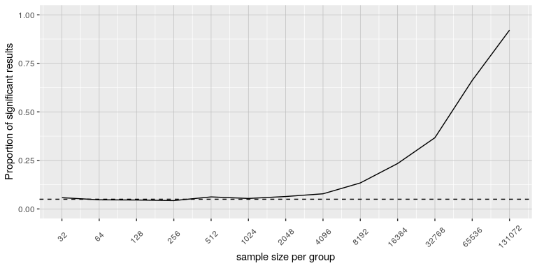
sample size and proportion of significant results, as sample size increases to over 4000, significant results increase dramatically

Figure 1: The proportion of significant results for a very small change (1 ounce, which is about .001 standard deviations) as a function of sample size.

Challenges with using p-values

Historically, the most common answer to this question has been that we should reject the null hypothesis if the p-value is less than 0.05. This comes from the writings of Ronald Fisher, who has been referred to as “the single most important figure in 20th century statistics” (Efron, 1998):

“If p is between .1 and .9 there is certainly no reason to suspect the hypothesis tested. If it is below .02 it is strongly indicated that the hypothesis fails to account for the whole of the facts. We shall not often be astray if we draw a conventional line at .05 … it is convenient to draw the line at about the level at which we can say: Either there is something in the treatment, or a coincidence has occurred such as does not occur more than once in twenty trials” (Fisher, 1925)

Fisher never intended p < 0.05 to be a fixed rule:

“no scientific worker has a fixed level of significance at which from year to year, and in all circumstances, he rejects hypotheses; he rather gives his mind to each particular case in the light of his evidence and his ideas” (Fisher, 1956)

Instead, it is likely that p < .05 became a ritual due to the reliance upon tables of p-values that were used before computing made it easy to compute p values for arbitrary values of a statistic. All of the tables had an entry for 0.05, making it easy to determine whether one’s statistic exceeded the value needed to reach that level of significance. Although we may use tables in this class, statistical software examines the specific probability value for the calculated statistic.

Assessing Error Rate: Type I and Type II Error

Although there are challenges with p-values for decision making, we will examine a way we can think about hypothesis testing in terms of its error rate. This was proposed by Jerzy Neyman and Egon Pearson:

“no test based upon a theory of probability can by itself provide any valuable evidence of the truth or falsehood of a hypothesis. But we may look at the purpose of tests from another viewpoint. Without hoping to know whether each separate hypothesis is true or false, we may search for rules to govern our behaviour with regard to them, in following which we insure that, in the long run of experience, we shall not often be wrong” (Neyman & Pearson, 1933)

That is: We can’t know which specific decisions are right or wrong, but if we follow the rules, we can at least know how often our decisions will be wrong in the long run.

To understand the decision-making framework that Neyman and Pearson developed, we first need to discuss statistical decision-making in terms of the kinds of outcomes that can occur. There are two possible states of reality (H0 is true, or H0 is false), and two possible decisions (reject H0, or retain H0). There are two ways in which we can make a correct decision:

We can reject H0 when it is false (in the language of signal detection theory, we call this a hit)
We can retain H0 when it is true (somewhat confusingly in this context, this is called a correct rejection)

There are also two kinds of errors we can make:

We can reject H0 when it is actually true (we call this a false alarm, or Type I error), Type I error means that we have concluded that there is a relationship in the population when in fact there is not. Type I errors occur because even when there is no relationship in the population, sampling error alone will occasionally produce an extreme result.
We can retain H0 when it is actually false (we call this a miss, or Type II error). Type II error means that we have concluded that there is no relationship in the population when in fact there is.

The Court Case Analogy Continued

Remember that a trial can end in two ways, much like hypothesis testing:

Guilty verdict = Reject the null hypothesis
- Strong evidence against innocence/null hypothesis
- Accept the alternative hypothesis
Not guilty verdict = Fail to reject the null hypothesis
- Insufficient evidence to prove guilt/alternative hypothesis
- We don’t prove innocence, we just lack evidence to reject it

There is a possibility for an error in the decision. We can make mistakes:

False conviction (Type I error) = Rejecting a true null hypothesis
False acquittal (Type II error) = Failing to reject a false null hypothesis

Summing up, when you perform a hypothesis test, there are four possible outcomes depending on the actual truth (or falseness) of the null hypothesis H0 and the decision to reject or not. The outcomes are summarized in the following table:

ACTION	H0 IS ACTUALLY
	True	False
Do not reject H0	Correct Outcome	Type II error
Reject H0	Type I Error	Correct Outcome

Table 1. The four possible outcomes in hypothesis testing.

The decision is not to reject H0 when H0 is true (correct decision).
The decision is to reject H0 when H0 is true (incorrect decision known as a Type I error).
The decision is not to reject H0 when, in fact, H0 is false (incorrect decision known as a Type II error).
The decision is to reject H0 when H0 is false (correct decision).

Neyman and Pearson coined two terms to describe the probability of these two types of errors in the long run:

P(Type I error) = αalpha
P(Type II error) = βbeta

That is, if we set αalpha to .05, then in the long run we should make a Type I error 5% of the time. The 𝞪 (alpha), is associated with the p-value for the level of significance. Again it’s common to set αalpha as .05. In fact, when the null hypothesis is true and α is .05, we will mistakenly reject the null hypothesis 5% of the time. (This is why α is sometimes referred to as the “Type I error rate.”) In principle, it is possible to reduce the chance of a Type I error by setting α to something less than .05. Setting it to .01, for example, would mean that if the null hypothesis is true, then there is only a 1% chance of mistakenly rejecting it. But making it harder to reject true null hypotheses also makes it harder to reject false ones and therefore increases the chance of a Type II error.

In practice, Type II errors occur primarily because the research design lacks adequate statistical power to detect the relationship (e.g., the sample is too small). Statistical power is the complement of Type II error. We will have more to say about statistical power shortly. The standard value for an acceptable level of β (beta) is .2 – that is, we are willing to accept that 20% of the time we will fail to detect a true effect when it truly exists. It is possible to reduce the chance of a Type II error by setting α to something greater than .05 (e.g., .10). But making it easier to reject false null hypotheses also makes it easier to reject true ones and therefore increases the chance of a Type I error. This provides some insight into why the convention is to set α to .05. There is some agreement among researchers that level of α keeps the rates of both Type I and Type II errors at acceptable levels.

The possibility of committing Type I and Type II errors has several important implications for interpreting the results of our own and others’ research. One is that we should be cautious about interpreting the results of any individual study because there is a chance that it reflects a Type I or Type II error. This is why researchers consider it important to replicate their studies. Each time researchers replicate a study and find a similar result, they rightly become more confident that the result represents a real phenomenon and not just a Type I or Type II error.

Test Statistic Assumptions

Last consideration we will revisit with each test statistic (e.g., t-test, z-test, and ANOVA) in the coming chapters. There are four main assumptions. These assumptions are often taken for granted in using prescribed data for the course. In the real world, these assumptions would need to be examined, often tested using statistical software.

Assumption of random sampling. A sample is random when each person (or animal) point in your population has an equal chance of being included in the sample; therefore selection of any individual happens by chance, rather than by choice. This reduces the chance that differences in materials, characteristics or conditions may bias results. Remember that random samples are more likely to be representative of the population so researchers can be more confident interpreting the results. Note: there is no test that statistical software can perform which assures random sampling has occurred but following good sampling techniques helps to ensure your samples are random.
Assumption of Independence. Statistical independence is a critical assumption for many statistical tests including the 2-sample t-test and ANOVA. It is assumed that observations are independent of each other often but often this assumption. Is not met. Independence means the value of one observation does not influence or affect the value of other observations. Independent data items are not connected with one another in any way (unless you account for it in your study). Even the smallest dependence in your data can turn into heavily biased results (which may be undetectable) if you violate this assumption. Note: there is no test statistical software can perform that assures independence of the data because this should be addressed during the research planning phase. Using a non-parametric test is often recommended if a researcher is concerned this assumption has been violated.
Assumption of Normality. Normality assumes that the continuous variables (dependent variable) used in the analysis are normally distributed. Normal distributions are symmetric around the center (the mean) and form a bell-shaped distribution. Normality is violated when sample data are skewed. With large enough sample sizes (n > 30) the violation of the normality assumption should not cause major problems (remember the central limit theorem) but there is a feature in most statistical software that can alert researchers to an assumption violation.
Assumption of Equal Variance. Variance refers to the spread or of scores from the mean. Many statistical tests assume that although different samples can come from populations with different means, they have the same variance. Equality of variance (i.e., homogeneity of variance) is violated when variances across different groups or samples are significantly different. Note: there is a feature in most statistical software to test for this.

Recap

We will use 4 main steps for hypothesis testing:

Begin with two hypotheses. Write a null hypothesis and alternative hypothesis about the populations.
1. Usually the hypotheses concern population parameters and predict the characteristics that a sample should have
2. The hypotheses are contradictory
  1. Null: Null hypothesis (H0) states that there is no difference, no effect or no change between population means and sample means. There is no difference.
  2. Alternative: Alternative hypothesis (H1 or HA) states that there is a difference or a change between the population and sample. It is the opposite of the null hypothesis.
Set criteria for a decision. In this step we must determine the boundary of our distribution at which the null hypothesis will be rejected. Researchers usually use either a 5% (.05) cutoff or 1% (.01) critical boundary. Recall from our earlier story about Ronald Fisher that the lower the probability the more confident the was that the Tea Lady was not guessing. We will apply this to z in the next chapter.
Sample data are collected and analyzed by performing statistics (calculations)
1. Compare sample and population to decide if the hypothesis has support
Make a decision and provide an explanation
1. When a researcher uses hypothesis testing, the individual is making a decision about whether the data collected is sufficient to state that the population parameters are significantly different.

Further considerations

The probability value is the probability of a result as extreme or more extreme given that the null hypothesis is true. It is the probability of the data given the null hypothesis. It is not the probability that the null hypothesis is false.
A low probability value indicates that the sample outcome (or one more extreme) would be very unlikely if the null hypothesis were true. We will learn more about assessing effect size later in this unit.
A non-significant outcome means that the data do not conclusively demonstrate that the null hypothesis is false. There is always a chance of error and 4 outcomes associated with hypothesis testing.

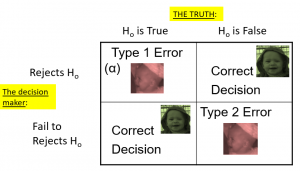decision with 4 possible outcomes for NHST image: author created

It is important to take into account the assumptions for each test statistic.

Learning objectives

Having read the chapter, you should be able to:

Identify the components of a hypothesis test, including the parameter of interest, the null and alternative hypotheses, and the test statistic.
State the hypotheses and identify appropriate critical areas depending on how hypotheses are set up.
Describe the proper interpretations of a p-value as well as common misinterpretations.
Distinguish between the two types of error in hypothesis testing, and the factors that determine them.
Describe the main criticisms of null hypothesis statistical testing
Identify the purpose of effect size and power.

Exercises – Ch. 9

In your own words, explain what the null hypothesis is.
What are Type I and Type II Errors?
What is α?
Why do we phrase null and alternative hypotheses with population parameters and not sample means?
If our null hypothesis is “H0: μ = 40”, what are the three possible alternative hypotheses?
Why do we state our hypotheses and decision criteria before we collect our data?
When and why do you calculate an effect size?

Answers to Odd- Numbered Exercises – Ch. 9

1. Your answer should include mention of the baseline assumption of no difference between the sample and the population.

3. Alpha is the significance level. It is the criteria we use when decided to reject or fail to reject the null hypothesis, corresponding to a given proportion of the area under the normal distribution and a probability of finding extreme scores assuming the null hypothesis is true.

5. μ > 40; μ < 40; μ ≠ 40

7. We calculate effect size to determine the strength of the finding. Effect size should always be calculated when the we have rejected the null hypothesis. Effect size can be calculated for non-significant findings as a possible indicator of Type II error.

License

Icon for the Creative Commons Attribution-NonCommercial-ShareAlike 4.0 International License

Introduction to Statistics for Psychology Copyright © 2021 by Alisa Beyer is licensed under a Creative Commons Attribution-NonCommercial-ShareAlike 4.0 International License, except where otherwise noted.