
13 Chapter 13: Independent Samples
We have seen how to compare a single mean against a given value and how to utilize difference scores to look for meaningful, consistent change via a single mean difference using a repeated measures design. Now, we will learn how to compare two separate means from separate groups that do not overlap to see if there is a difference between them. The process of testing hypotheses about two means is exactly the same as it is for testing hypotheses about a single mean, and the logical structure of the formulae is the same as well. However, we will be adding a few extra steps this time to account for the fact that our data are coming from different sources.
Difference of Means
Last chapter, we learned about mean differences, that is, the average value of difference scores. Those difference scores came from ONE group and TWO time points (or two perspectives). Now, we will deal with the difference of the means, that is, the average values of separate groups that are represented by separate descriptive statistics. This analysis involves TWO groups and ONE time point. As with all of our other tests as well, both of these analyses are concerned with a single variable.
It is very important to keep these two tests separate and understand the distinctions between them because they assess very different questions and require different approaches to the data. When in doubt, think about how the data were collected and where they came from. If they came from two time points with the same people (sometimes referred to as “longitudinal” data), you know you are working with repeated measures data (the measurement literally was repeated) and will use a paired/dependent samples t-test. If it came from a single time point that used separate groups, you need to look at the nature of those groups and if they are related. Can individuals in one group being meaningfully matched up with one and only one individual from the other group? For example, are they a romantic couple? If so, we call those data matched and we use a matched pairs/dependent samples t-test. However, if there’s no logical or meaningful way to link individuals across groups, or if there is no overlap between the groups, then we say the groups are independent and use the independent samples t-test, the subject of this chapter.
Research Questions about Independent Means
An independent samples t-test is also designed to compare populations. If we want to know if two populations differ and we do not know the mean of either population, we take a sample from each and then conduct an independent sample t-test. Many research ideas in the behavioral sciences and other areas of research are concerned with whether or not two means are the same or different. Logically, we can then say that these research questions are concerned with group mean differences. That is, on average, do we expect a person from Group A to be higher or lower on some variable that a person from Group B. In any time of research design looking at group mean differences, there are some key criteria we must consider: the groups must be mutually exclusive (i.e. you can only be part of one group at any given time) and the groups have to be measured on the same variable (i.e. you can’t compare personality in one group to reaction time in another group since those values would not be the same anyway).
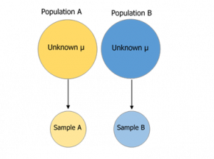
Figure 1. Collecting data from 2 different groups.
If the difference between the sample means given in the problem is very large compared to the differences we would expect to see between samples drawn from the same population, then we will conclude that the two samples must be from different populations. The language of the two independent samples t-tests involves probability statements because we know that there is variability in the samples that we draw from populations. If we were to draw two samples from a particular population we would expect a difference between the means of the samples by chance alone. In an independent sample situation we are given two sample means and understand that they are probably not equal BUT this does NOT provide evidence that the samples are from different populations. In independent samples t-tests we must estimate the probability of drawing particular differences between sample means from a population before deciding whether the difference between the sample means given in the problem is sufficiently large to lead us to conclude that the samples must be from different populations.
As we can see, the grouping variable we use for an independent samples t-test can be a set of groups we create (as in the experimental medication example) or groups that already exist naturally (as in the university example). There are countless other examples of research questions relating to two group means, making the independent samples t-test one of the most widely used analyses around.

 Photo credit We know can say tea for two, as the saying goes, one for me and one for you, is for two different people having tea at the same time. This follows the independent t-test having two separate groups at the same time point.
Setting up step 1
In chapter 12, it is the same participants tracked over 2 timepoints for the paired samples t-test. This is an example of a repeated measures or within-group design. This chapter focuses on two different samples compared, using independent samples t-test, known as a between-group design. In setting up step 1, there will be a few variations to how to set up the null and alternative (H1 or HA) hypotheses. You can see these are all ways to set up the two types of research hypotheses (three hypotheses for the 2 directional and 1 for the non-directional). You can set it up by comparing both groups (first 2 columns) or examining differences (which is similar to how we set up the top of your t-formula).
|
Research Question |
Hypotheses in 3 ways | ||
| Are male scores higher than female scores?
(between-group design) |
H0: μM – μF ≤ 0 H1: μM – μF > 0 |
in other words:
H0: μM ≤ μF H1: μM > μF |
in other words:
H0: μM ≤ μF H1: μM > μF |
| Are male scores lower than female scores?
(between-group design) |
H0: μM – μF ≥ 0
H1: μM – μF < 0
|
in other words:
H0: μM ≥ μF H1: μM < μF |
in other words: H0: μM ≥ μF H1: μM < μF
|
| Are male scores different from female scores?
(between-group design) |
H0: μM – μF= 0
H1: μM – μF ≠ 0
|
in other words:
H0: μM = μF H1 μM ≠ μF |
in other words: H0: μM = μF H1: μM ≠ μF
|
| Do athlete performance improve after training?
(within-group design) |
H0: μD ≤ 0
H1: μD > 0 |
in other words: H0: μ1 ≤ μ2 H1: μ1 > μ2 |
in other words:
H0: μ1 – μ2 ≤ 0 H1: μ1 – μ2 > 0 |
| Do athlete reaction times decrease after training?
(within-group design) |
H0: μD ≥ 0 H1: μD < 0 |
in other words:
H0: μ1 ≥ μ2 H1: μ1 < μ2 |
in other words:
H0: μ1 – μ2 ≥ 0 H1: μ1 – μ2 < 0 |
| Does training have an effect on athlete reaction times?
(within-group design) |
H0: μD = 0 H1: μD ≠ 0 |
in other words:
H0: μ1 = μ2 H1 μ1 ≠ μ2 |
in other words:
H0: μ1 – μ2= 0 H1: μ1 – μ2 ≠ 0 |
Table 1. Examples of hypotheses set up for 2 samples based on between-group and within-group design.
Hypotheses and Decision Criteria
The process of testing hypotheses using an independent samples t-test is the same as it was in the last three chapters, and it starts with stating our hypotheses and laying out the criteria we will use to test them.
Our alternative hypotheses are also unchanged: we simply replace the equal sign (=) with one of the three inequalities (>, <, ≠):
HA: µ1 > µ2 or µ1 − µ2 > 0; HA: Group 1 is more than/stronger than group 2.
HA: µ1 < µ2 or µ1 − µ2 < 0; HA: Group 1 is less than/weaker than group 2.
HA: µ1 ≠ µ2 or µ1 − µ2 ≠ 0; HA: There is no difference between the two groups.
H0: There is no difference between the means of the treatment (T) and control (C) groups. H0: µT = µC
HA: There is a difference between the means of the treatment (T) and control (C) group. HA: µT ≠ µC
Step 2
Once we have our hypotheses laid out, we can set our criteria to test them using the same three pieces of information as before: significance level (α), directionality (left, right, or two-tailed), and degrees of freedom. We will use the same critical value t table, but a new degrees of freedom for the independent samples t-test.
This looks different than before, but it is just adding the individual degrees of freedom from each group (n – 1) together. Notice that the sample sizes, n, also get subscripts so we can tell them apart. For an independent samples t-test, it is often the case that our two groups will have slightly different sample sizes, either due to chance or some characteristic of the groups themselves. Generally, this is not as issue, so long as one group is not massively larger than the other group, and there are not large differences in the variance of each group (more on this later).
Independent Samples t-statistic
The test statistic for our independent samples t-test takes on the same logical structure and format as our other t-tests: our observed effect minus our null hypothesis value, all divided by the standard error:
Independent samples t-test

M1 is the sample mean for group 1 and M2 is the sample mean for group 2. This looks like more work to calculate, but remember that our null hypothesis states that the quantity μ1 – μ2 = 0, so we can drop that out of the equation and are left with:

Our standard error in the denominator (bottom of the formula) is denoting what it is the standard error of (derived from 2 samples). Because we are dealing with the difference between two separate means, rather than a single mean or single mean of difference scores, we put both means in the subscript.
Calculating our standard error, as we will see next, is where the biggest differences between this t-test and other t-tests appears. However, once we do calculate it and use it in our test statistic, everything else goes back to normal. Our decision criteria is still comparing our obtained test statistic to our critical value, and our interpretation based on whether or not we reject the null hypothesis is unchanged as well.
Standard Error and Pooled Variance
Recall that the standard error is the average distance between any given sample mean and the center of its corresponding sampling distribution, and it is a function of the standard deviation of the population (either given or estimated) and the sample size. This definition and interpretation hold true for our independent samples t-test as well, but because we are working with two samples drawn from two populations, we have to first combine their estimates of standard deviation – or, more accurately, their estimates of variance – into a single value that we can then use to calculate our standard error.
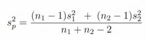
The combined estimate of variance using the information from each sample is called the pooled variance and is denoted Sp2; the subscript p serves as a reminder indicating that it is the pooled variance. The term “pooled variance” is a literal name because we are simply pooling or combining the information on variance – the Sum of Squares and Degrees of Freedom – from both of our samples into a single number. The result is a weighted average of the observed sample variances, the weight for each being determined by the sample size, and will always fall between the two observed variances. The computational formula for the pooled variance is:
Pooled variance used to get to our new standard error formula
 This formula can look daunting at first, but it is in fact just a weighted average. Even more conveniently, some simple algebra can be employed to greatly reduce the complexity of the calculation. The simpler and more appropriate formula to use when calculating pooled variance is:
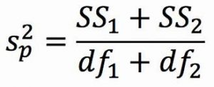
Both formula will give you the same pooled variance. The most common formula used is the SS/df (which is how we typically think about variance). Using the SS/df formula, it’s very simple to see that we are just adding together the same pieces of information we have been calculating since chapter 3.
Once we have our pooled variance calculated, we can drop it into the equation for our standard error:
Standard error for independent t-test 
Once again, although this formula may seem different than it was before, in reality it is just a different way of writing the same thing. Think back to the standard error options presented in chapter 9, when our standard error was
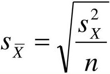
Looking at that, we can now see that, once again, we are simply adding together two pieces of information: no new logic or interpretation required. Once the standard error is calculated, it goes in the denominator of our test statistic, as shown above and as was the case in all previous chapters. Thus, the only additional step to calculating an independent samples t-statistic is computing the pooled variance. Let’s see an example in action.
Example: Movies and Mood
We are interested in whether the type of movie someone sees at the theater affects their mood when they leave. We decide to ask people about their mood as they leave one of two movies: a comedy (group 1, n = 35) or a horror film (group 2, n = 29). Our data are coded so that higher scores indicate a more positive mood. We have good reason to believe that people leaving the comedy will be in a better mood, so we use a one-tailed test at α = 0.05 to test our hypothesis.
Step 1: State the Hypotheses
As always, we start with hypotheses:
H0: There is no difference in average mood between the two movie types
H0: μ1 – μ2 = 0 or H0: μ1 = μ2
HA: The comedy film will give a better average mood than the horror film
HA: μ1 – μ2 > 0 or HA: μ1 > μ2
Notice that in the first formulation of the alternative hypothesis we say that the first mean minus the second mean will be greater than zero. This is based on how we code the data (higher is better), so we suspect that the mean of the first group will be higher. Thus, we will have a larger number minus a smaller number, which will be greater than zero. Be sure to pay attention to which group is which and how your data are coded (higher is almost always used as better outcomes) to make sure your hypothesis makes sense!
Step 2: Find the Critical Values
Just like before, we will need critical values, which come from out t-table. In this example, we have a one-tailed test at α = 0.05 and expect a positive answer (because we expect the difference between the means to be greater than zero). Our degrees of freedom for our independent samples t-test is just the degrees of freedom from each group added together: 35 + 29 – 2 = 62. From our t-table, we find that our critical value is t* = 1.671. Note: because 62 does not appear on the critical values table, we use the next lowest value, which in this case is 60.
Step 3: Compute the Test Statistic
The data from our two groups are presented in the tables below. Table 1 shows the summary values for the Comedy group, and Table 2 shows the summary values for the Horror group (the end of the chapter contains the raw data).
|
Group 1: Comedy Film |
||
|
n |
M |
SS |
|
35 |
ΣX/n = 840/35 |
Σ(X − ̅X)2=5061.60 |
Table 1. Raw scores and Sum of Squares for Group 1
|
Group 2: Horror Film |
||
|
n |
M |
SS |
| 29 | ΣX/n = 478.6/29 = 16.5 | Σ(X − ̅X)2 = 3896.45 |
Table 2. Raw scores and Sum of Squares for Group 1.
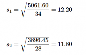
the Sum of Squares for each group: SS1 = 5061.60 and SS2 = 3896.45. These values have all been calculated and take on the same interpretation as they have since chapter 3. Before we move on to the pooled variance that will allow us to calculate standard error, let’s compute our standard deviation for each group; even though we will not use them in our calculation of the test statistic, they are still important descriptors of our data:
Now we can move on to our new calculation, the pooled variance, which is just the Sums of Squares that we calculated from our table and the degrees of freedom, which is just n – 1 for each group:
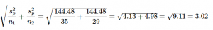
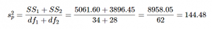 As you can see, if you follow the regular process of calculating standard deviation using the Sum of Squares table, finding the pooled variance is very easy. Now we can use that value to calculate our standard error, the last step before we can find our test statistic:
Now we can move on to the final step of the hypothesis testing procedure.
Step 4: Make the Decision
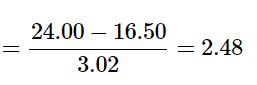
Our test statistic has a value of t = 2.48, and in step 2 we found that the critical value is t* = 1.671. 2.48 > 1.671, so we reject the null hypothesis:
Reject H0. Based on our sample data from people who watched different kinds of movies, we can say that the average mood after a comedy movie (M2= 24.00) is better than the average mood after a horror movie (M2 = 16.50), t(62) = 2.48, p < .05.
Effect Sizes and Confidence Intervals
We have seen in previous chapters that even a statistically significant effect needs to be interpreted along with an effect size to see if it is practically meaningful. We have also seen that our sample means, as a point estimate, are not perfect and would be better represented by a range of values that we call a confidence interval. As with all other topics, this is also true of our independent samples t-tests. Our effect size for the independent samples t-test is still Cohen’s d, and it is still just our observed effect divided by the standard deviation. Remember that standard deviation is just the square root of the variance, and because we work with pooled variance in our test statistic, we will use the square root of the pooled variance as our denominator in the formula for Cohen’s d. We also can still calculate r2, the percentage of variance accounted from by the independent variable/treatment effect.
 Just like chapter 12, you also have r2 as an option.
 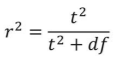 where df is the df calculated in step 2. The r2 is interpreted as percent of variance in the dependent variable accounted from by the independent variable. Remember that r2 is calculated when you have an effect.
For our example above, M1 = 24, M2 = 16.5, sp2 = 144.48, we can calculate Cohen’s d to be:
d =24-16.50/√(144.48)=7.5/12.02 = 0.62
We interpret this using the same guidelines as before, so we would consider this a moderate or moderately large effect.
For our example above, t = 2.48 (thus t2 = 2.48*2.48= 6.15), df = 62, we can calculate r2 to be:
r2 = 6.15/(6.15+62) = 6.15/68.15 = 0.09
We interpret this using the same guidelines as before, so 9% of the variance in mood (our DV) is from type of movie (our IV).
Our confidence intervals also take on the same form and interpretation as they have in the past. The value we are interested in is the difference between the two means, so our point estimate is the value of one mean minus the other, or M1 – M2. Just like before, this is our observed effect and is the same value as the one we place in the numerator of our test statistic. We calculate this value then place the margin of error – still our critical value times our standard error – above and below it.
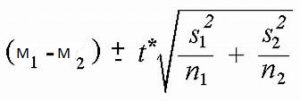 where you would still calculate upper bound (UB) and lower bound (LB) values with t being the critical value t-value using a 2-tail test.
Because our hypothesis testing example used a one-tailed test, it would be inappropriate to calculate a confidence interval on those data (remember that we can only calculate a confidence interval for a two-tailed test because the interval extends in both directions).
Example: Confidence Interval
Let’s say we find summary statistics on the average life satisfaction of people from two different towns and want to create a confidence interval to see if the difference between the two might actually be zero.
Our sample data are M1 = 28.65 s1 = 12.40 n1 = 40 and M2 = 25.40, s2 = 15.68 n2 = 42. At face value, it looks like the people from the first town have higher life satisfaction (28.65 vs. 25.40), but it will take a confidence interval (or complete hypothesis testing process) to see if that is true or just due to random chance.
First, we want to calculate the difference between our sample means, which is 28.65 –25.40 = 3.25.
Next, we need a critical value from our t-table. If we want to test at the normal 95% level of confidence, then our sample sizes will yield degrees of freedom equal to 40 + 42 – 2 = 80. From our table, that gives us a critical value of t* = 1.990.
Finally, we need our standard error. Recall that our standard error for an independent samples t-test uses pooled variance, which requires the Sum of Squares and degrees of freedom. Up to this point, we have calculated the Sum of Squares using raw data, but in this situation, we do not have access to it. So, what are we to do?
If we have summary data like standard deviation and sample size, it is very easy to calculate the pooled variance using the other formula presented
If s1 = 12.40, then s12 = 12.40*12.40 = 153.76, and if s2 = 15.68, then s22 = 15.68*16.68 = 245.86. With n1 = 40 and n2 = 42, we are all set to calculate the pooled variance.
sp2 = [(40-1)(153.76) + (42-1)(245.86)]/(40+42-2) = [(39)(153.76) + (41)(245.86)]/80 = (5996.64 + 10080.36)/80 =16077/80 = 200.96
Plugging in sp2 = 200.96, n1 = 40, and n2 = 42nd, our standard error equals:
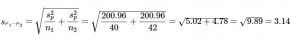
All of these steps are just slightly different ways of using the same formulae, numbers, and ideas we have worked with up to this point. Once we get out standard error, it’s time to build our confidence interval.
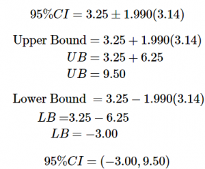
Our confidence interval, as always, represents a range of values that would be considered reasonable or plausible based on our observed data. In this instance, our interval (-3.00, 9.50) does contain zero. Thus, even though the means look a little bit different, it may very well be the case that the life satisfaction in both of these towns is the same. Proving otherwise would require more data.
Hypothesis testing and confidence intervals
As mentioned when confidence intervals where introduced, there is a close relationship between confidence intervals and hypothesis tests. In particular, if the confidence interval does not include the null hypothesis, then the associated statistical test would be statistically significant. However, things get trickier if we want to compare the means of two conditions (Schenker and Gentleman, 2001). There are a couple of situations that are clear. First, if each mean is contained within the confidence interval for the other mean, then there is definitely no significant difference at the chosen confidence level. Second, if there is no overlap between the confidence intervals, then there is certainly a significant difference at the chosen level; in fact, this test is substantially conservative, such that the actual error rate will be lower than the chosen level. But what about the case where the confidence intervals overlap one another but don’t contain the means for the other group? In this case the answer depends on the relative variability of the two variables, and there is no general answer. However, one should in general avoid using the “eyeball test” for overlapping confidence intervals.
Homogeneity of Variance
Before wrapping up the coverage of independent samples t-tests, there is one other important topic to cover. Using the pooled variance to calculate the test statistic relies on an assumption known as homogeneity of variance. In statistics, an assumption is some characteristic that we assume is true about our data, and our ability to use our inferential statistics accurately and correctly relies on these assumptions being true. If these assumptions are not true, then our analyses are at best ineffective (e.g. low power to detect effects) and at worst inappropriate (e.g. too many Type I errors). A detailed coverage of assumptions is beyond the scope of this course, but it is important to know that they exist for all analyses.
Review: Statistical Power
There are three factors that can affect statistical power:
- Sample size: Larger samples provide greater statistical power
- Effect size: A given design will always have greater power to find a large effect than a small effect (because finding large effects is easier)
- Type I error rate: There is a relationship between Type I error and power such that (all else being equal) decreasing Type I error will also decrease power.
We can see this through simulation. First let’s simulate a single experiment, in which we compare the means of two groups using a standard t-test. We will vary the size of the effect (specified in terms of Cohen’s d), the Type I error rate, and the sample size, and for each of these we will examine how the proportion of significant results (i.e. power) is affected. Figure 1 shows an example of how power changes as a function of these factors.
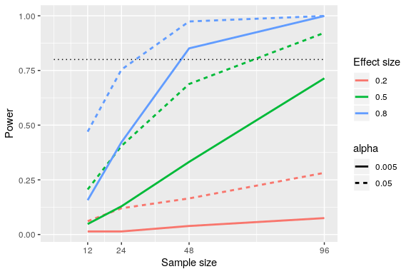
Figure 1: Results from power simulation, showing power as a function of sample size, with effect sizes shown as different colors, and alpha shown as line type. The standard criterion of 80 percent power is shown by the dotted black line.
This simulation shows us that even with a sample size of 96, we will have relatively little power to find a small effect (d=0.2d = 0.2) with α=0.005\alpha = 0.005. This means that a study designed to do this would be futile – that is, it is almost guaranteed to find nothing even if a true effect of that size exists.
There are at least two important reasons to care about statistical power. First, if you are a researcher, you probably don’t want to spend your time doing futile experiments. Running an underpowered study is essentially futile, because it means that there is a very low likelihood that one will find an effect, even if it exists. Second, it turns out that any positive findings that come from an underpowered study are more likely to be false compared to a well-powered study, a point we discuss in more detail in Chapter 19. Fortunately, there are tools available that allow us to determine the statistical power of an experiment. The most common use of these tools is in planning an experiment, when we would like to determine how large our sample needs to be in order to have sufficient power to find our effect of interest.
Assumptions of independent t-test
Assumptions are conditions that must be met in order for our hypothesis testing conclusion to be valid. [Important: If the assumptions are not met then our hypothesis testing conclusion is not likely to be valid. Testing errors can still occur even if the assumptions for the test are met.]
Recall that inferential statistics allow us to make inferences (decisions, estimates, predictions) about a population based on data collected from a sample. Recall also that an inference about a population is true only if the sample studied is representative of the population. A statement about a population based on a biased sample is not likely to be true.
Assumption 1: Individuals in the sample were selected randomly and independently, so the sample is highly likely to be representative of the larger population.
- Random sampling ensures that each member of the population is equally likely to be selected.
- An independent sample is one which the selection of one member has no effect on the selection of any other.
Assumption 2: The distribution of sample differences (DSD) is a normal, because we drew the samples from a population that was normally distributed.
- This assumption is very important because we are estimating probabilities using the t- table – which provide accurate estimates of probabilities for events distributed normally.
Assumption 3: Sampled populations have equal variances or have homogeneity of variance.
Learning Objectives
Having read this chapter, a student should be able to:
- Identify under what study design to use an independent t-test
- Use the independent t-test to test hypotheses about mean differences between two populations or treatment conditions
- Calculate and evaluate effect size options, Cohen’s d and r2
Exercises – Ch. 13
- What is meant by “the difference of the means” when talking about an independent samples t-test? How does it differ from the “mean of the differences” in a repeated measures t-test?
- Describe three research questions that could be tested using an independent samples t-test.
- Calculate pooled variance from the following raw data:
|
Group 1 |
Group 2 |
| 16 | 4 |
| 11 | 10 |
|
9 |
15 |
|
7 |
13 |
|
5 |
12 |
|
4 |
9 |
| 12 |
8 |
4. Calculate the standard error from the following descriptive statistics
- s1 = 24, s2 = 21, n1 = 36, n2 = 49
- s1 = 15.40, s2 = 14.80, n1 = 20, n2 = 23
- s1 = 12, s2 = 10, n1 = 25, n2 = 25
5. Determine whether to reject or fail to reject the null hypothesis in the following situations:
- t(40) = 2.49, α = 0.01, one-tailed test to the right
- X̅̅̅ = 64, ̅X̅̅̅ = 54, n1 = 14, n2 = 12, 𝑠̅̅̅̅ ̅̅̅̅ = 9.75, α = 0.05, two-tailed test
- 95% Confidence Interval: (0.50, 2.10)
6. A professor is interest in whether or not the type of software program used in a statistics lab affects how well students learn the material. The professor teaches the same lecture material to two classes but has one class use a point-and-click software program in lab and has the other class use a basic programming language. The professor tests for a difference between the two classes on their final exam scores.
|
Point-and-Click |
Programming |
|
83 |
86 |
|
83 |
79 |
|
63 |
100 |
|
77 |
74 |
|
86 |
70 |
|
84 |
67 |
|
78 |
83 |
|
61 |
85 |
|
65 |
74 |
|
75 |
86 |
|
100 |
87 |
|
60 |
61 |
|
90 |
76 |
|
66 |
100 |
|
54 |
|
7. A researcher wants to know if there is a difference in how busy someone is based on whether that person identifies as an early bird or a night owl. The researcher gathers data from people in each group, coding the data so that higher scores represent higher levels of being busy, and tests for a difference between the two at the .05 level of significance.
|
Early Bird |
Night Owl |
|
23 |
26 |
|
28 |
10 |
|
27 |
20 |
|
33 |
19 |
|
26 |
26 |
|
30 |
18 |
|
22 |
12 |
|
25 |
25 |
|
26 |
|
8. Lots of people claim that having a pet helps lower their stress level. Use the following summary data to test the claim that there is a lower average stress level among pet owners (group 1) than among non-owners (group 2) at the .05 level of significance. M1 = 16.25, M2 = 20.95, s1 = 4.00, s2 = 5.10, n1 = 29, n2 = 25
9. Administrators at a university want to know if students in different majors are more or less extroverted than others. They provide you with descriptive statistics they have for English majors (coded as 1) and History majors (coded as 2) and ask you to create a confidence interval of the difference between them. Does this confidence interval suggest that the students from the majors differ? M1 = 3.78, M2= 2.23, s1 = 2.60, s2 = 1.15, n1 = 45, n2 = 40
10. Researchers want to know if people’s awareness of environmental issues varies as a function of where they live. The researchers have the following summary data from two states, Alaska and Hawaii, that they want to use to test for a difference. MH = 47.50, MA = 45.70, sH = 14.65, sA = 13.20, nH = 139, nA = 150
Answers to Odd- Numbered Exercises – Ch. 13
1. The difference of the means is one mean, calculated from a set of scores, compared to another mean which is calculated from a different set of scores; the independent samples t-test looks for whether the two separate values are different from one another. This is different than the “mean of the differences” because the latter is a single mean computed on a single set of difference scores that come from one data collection of matched pairs. So, the difference of the means deals with two numbers but the mean of the differences is only one number.
9. M1-M2 = 1.55, t* = 1.990, sM1-M2= 0.45, CI = (0.66, 2.44). This confidence interval does not contain zero, so it does suggest that there is a difference between the extroversion of English majors and History majors.
Raw scores from the mood and movies example
|
Group 1: Comedy Film |
||
|
X |
(X − ̅X) |
(X − ̅X)2 |
|
39.10 |
15.10 |
228.01 |
|
38.00 |
14.00 |
196.00 |
|
14.90 |
-9.10 |
82.81 |
|
20.70 |
-3.30 |
10.89 |
|
19.50 |
-4.50 |
20.25 |
|
32.20 |
8.20 |
67.24 |
|
11.00 |
-13.00 |
169.00 |
|
20.70 |
-3.30 |
10.89 |
|
26.40 |
2.40 |
5.76 |
|
35.70 |
11.70 |
136.89 |
|
26.40 |
2.40 |
5.76 |
|
28.80 |
4.80 |
23.04 |
|
33.40 |
9.40 |
88.36 |
|
13.70 |
-10.30 |
106.09 |
|
46.10 |
22.10 |
488.41 |
|
13.70 |
-10.30 |
106.09 |
|
23.00 |
-1.00 |
1.00 |
|
20.70 |
-3.30 |
10.89 |
|
19.50 |
-4.50 |
20.25 |
|
11.40 |
-12.60 |
158.76 |
|
24.10 |
0.10 |
0.01 |
|
17.20 |
-6.80 |
46.24 |
|
38.00 |
14.00 |
196.00 |
|
10.30 |
-13.70 |
187.69 |
|
35.70 |
11.70 |
136.89 |
|
41.50 |
17.50 |
306.25 |
|
18.40 |
-5.60 |
31.36 |
|
36.80 |
12.80 |
163.84 |
|
54.10 |
30.10 |
906.01 |
|
11.40 |
-12.60 |
158.76 |
|
8.70 |
-15.30 |
234.09 |
|
23.00 |
-1.00 |
1.00 |
|
14.30 |
-9.70 |
94.09 |
|
5.30 |
-18.70 |
349.69 |
|
6.30 |
-17.70 |
313.29 |
|
Σ = 840 |
Σ = 0 |
Σ=5061.60 |
|
Group 2: Horror Film |
||
|
X |
(X − ̅X) |
(X − ̅X)2 |
|
24.00 |
7.50 |
56.25 |
|
17.00 |
0.50 |
0.25 |
|
35.80 |
19.30 |
372.49 |
|
18.00 |
1.50 |
2.25 |
|
-1.70 |
-18.20 |
331.24 |
|
11.10 |
-5.40 |
29.16 |
|
10.10 |
-6.40 |
40.96 |
|
16.10 |
-0.40 |
0.16 |
|
-0.70 |
-17.20 |
295.84 |
|
14.10 |
-2.40 |
5.76 |
|
25.90 |
9.40 |
88.36 |
|
23.00 |
6.50 |
42.25 |
|
20.00 |
3.50 |
12.25 |
|
14.10 |
-2.40 |
5.76 |
|
-1.70 |
-18.20 |
331.24 |
|
19.00 |
2.50 |
6.25 |
|
20.00 |
3.50 |
12.25 |
|
30.90 |
14.40 |
207.36 |
|
30.90 |
14.40 |
207.36 |
|
22.00 |
5.50 |
30.25 |
|
6.20 |
-10.30 |
106.09 |
|
27.90 |
11.40 |
129.96 |
|
14.10 |
-2.40 |
5.76 |
|
33.80 |
17.30 |
299.29 |
|
26.90 |
10.40 |
108.16 |
|
5.20 |
-11.30 |
127.69 |
|
13.10 |
-3.40 |
11.56 |
|
19.00 |
2.50 |
6.25 |
|
-15.50 |
-32.00 |
1024.00 |
|
Σ = 478.6 |
Σ = 0.10 |
Σ=3896.45 |
Table 1. Raw scores and Sum of Squares for Group 1
Table 2. Raw scores and Sum of Squares for Group 2.
