
4 Chapter 4: Measures of Central Tendency
Now that we have visualized our data to understand its shape, we can begin with numerical analyses! The descriptive statistics presented in this chapter serve to start to describe the distribution of our data objectively and mathematically – our first step into statistical analysis! The topics here will serve as the basis for everything we do in the rest of the course.
Review: There are four different scales of measurement that go along with these different ways that values of a variable can differ.
Nominal scale. A nominal variable satisfies the criterion of identity, such that each value of the variable represents something different, but the numbers simply serve as qualitative labels as discussed above. For example, we might ask people for their political party affiliation, and then code those as numbers: 1 = “Republican”, 2 = “Democrat”, 3 = “Libertarian”, and so on. However, the different numbers do not have any ordered relationship with one another.
Ordinal scale. An ordinal variable satisfies the criteria of identity and magnitude, such that the values can be ordered in terms of their magnitude. For example, we might ask a person with chronic pain to complete a form every day assessing how bad their pain is, using a 1-7 numeric scale. Note that while the person is presumably feeling more pain on a day when they report a 6 versus a day when they report a 3, it wouldn’t make sense to say that their pain is twice as bad on the former versus the latter day; the ordering gives us information about relative magnitude, but the differences between values are not necessarily equal in magnitude.
Interval scale. An (equal) interval scale has all of the features of an ordinal scale, but in addition, the intervals between units on the measurement scale can be treated as equal. A standard example is physical temperature measured in Celsius or Fahrenheit; the physical difference between 10 and 20 degrees is the same as the physical difference between 90 and 100 degrees, but each scale can also take on negative values.
Ratio scale. A ratio scale variable has all four of the features outlined above: identity, magnitude, equal intervals, and absolute zero. The difference between a ratio scale variable and an interval scale variable is that the ratio scale variable has a true zero point. Examples of ratio scale variables include physical height and weight, along with temperature measured in Kelvin.
There are two important reasons that we must pay attention to the scale of measurement of a variable. First, the scale determines what kind of mathematical operations we can apply to the data (see Table 1). A nominal variable can only be compared for equality; that is, do two observations on that variable have the same numeric value? It would not make sense to apply other mathematical operations to a nominal variable, since they don’t really function as numbers in a nominal variable, but rather as labels. With ordinal variables, we can also test whether one value is greater or lesser than another, but we can’t do any arithmetic. Interval and ratio variables allow us to perform arithmetic; with interval variables we can only add or subtract values, whereas with ratio variables we can also multiply and divide values.
| Equal/not equal | >/< | +/- | Multiply/divide | |
|---|---|---|---|---|
| Nominal | OK | |||
| Ordinal | OK | OK | ||
| Interval | OK | OK | OK | |
| Ratio | OK | OK | OK | OK |
These constraints also imply that there are certain kinds of statistics that we can compute on each type of variable. Statistics that simply involve counting different values (such as the most common value, known as the mode), can be calculated on any of the variable types. Other statistics are based on ordering or ranking of values (such as the median, which is the middle value when all of the values are ordered by their magnitude), and these require that the value at least be on an ordinal scale. Finally, statistics that involve adding up values (such as the average, or mean), require that the variables be at least on an interval scale. Having said that, we should note that it’s quite common for researchers to compute the mean of variables that are only ordinal (such as responses on personality tests), but this can sometimes be problematic.
What is Central Tendency?
Therefore, a measure of central tendency is a way to summarize a large set of numbers using one single score. We can use measures of central tendency to describe a single distribution or compare multiple sets of scores but we have to figure out which measure of central tendency best represents a given distribution.
You might be thinking this is simple. After all, finding the “center” of a distribution involves just looking at it but let’s look at the 3 frequency distributions below and decide subjectively what the most typical or representative “center” score would be.
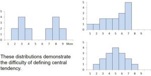
Figure 1. Three different distributions
These distributions demonstrate that finding the center of a distribution may be more challenging than first thought.
Let’s consider another example. Imagine this situation: You are in a class with just four other students, and the five of you took a 5-point pop quiz. Today your instructor is walking around the room, handing back the quizzes. She stops at your desk and hands you your paper.
In Dataset A, everyone’s score is 3. This puts your score at the exact center of the distribution. You can draw satisfaction from the fact that you did as well as everyone else. But of course, it cuts both ways: everyone else did just as well as you.
|
Student |
Dataset A |
Dataset B |
Dataset C |
|
You |
3 |
3 |
3 |
|
John’s |
3 |
4 |
2 |
|
Maria’s |
3 |
4 |
2 |
|
Shareecia’s |
3 |
4 |
2 |
|
Luther’s |
3 |
5 |
1 |
Table 2. Three possible datasets for the 5-point make-up quiz.
Now let’s change the example in order to develop more insight into the center of a distribution. For this example, there is a quasi-experiment with 2 groups (levels of the IV), tournament players and novices (people who don’t play chess). Subjects were shown a chess position and then asked to reconstruct it on an empty chessboard. The number of pieces correctly placed was recorded for three chess positions. The scores represent the total number of chess pieces correctly placed for the three chess positions (the DV). The maximum possible score was 89. Figure 2 shows the results of an experiment on memory for chess positions. This is a type of stem and leaf plot called a back-to-back stemplot. There are two groups being compared. On the left are people who don’t play chess (novice). On the right are people who play a great deal (tournament players). It is clear that the location of the center of the distribution for the non-players is much lower than the center of the distribution for the tournament players.
novice tournament players
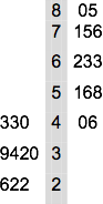
Figure 2. Back-to-back stem and leaf display. The left side shows the memory scores of the non-players. The right side shows the scores of the tournament players.
There turn out to be (at least) three different ways of thinking about the center of a distribution, all of them useful in various contexts. In the remainder of this section, we will give statistical measures for these concepts of central tendency. These are the three measures of central tendency:
- Mean
- Median
- Mode
Mean
One definition of central tendency is the point at which the distribution is in balance. Figure 3 shows the distribution of the five numbers 2, 3, 4, 9, 16 placed upon a balance scale. If each number weighs one pound, and is placed at its position along the number line, then it would be possible to balance them by placing a fulcrum at 6.8. The fulcrum or balancing point is calculated as the arithmetic mean or mean.
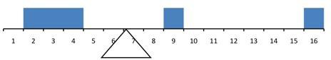
Figure 3. A balance scale demonstrating the mean as the fulcrum.
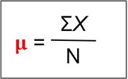
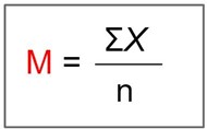
The arithmetic mean is the most common measure of central tendency. The mean is essentially the balancing point of a distribution of scores. This means the distance to all scores below the mean equals the distance to all scores above the mean. The mathematical definition of the mean is the point in a distribution at which the total distance to all the scores above that point equals the total distance to all scores below that point. It is simply the sum of the numbers divided by the number of numbers. The symbol “μ” (pronounced “mew”) is used for the mean of a population. The symbol “̅X” (pronounced “X-bar”) or M is used for the mean of a sample.
Mean
The formula for μ (population) and 𝑋̅ or M (sample):
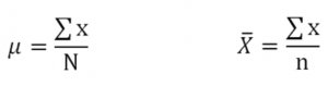
For the μ formula, ΣX is the sum of all the numbers in the population and N is the number of numbers in the population. The formula for 𝑋̅ or M is essentially identical where ΣX is the sum of all the numbers in the sample and n is the number of numbers in the sample.
The only distinction between these two equations is whether we are referring to the population (in which case we use the parameter μ) or a sample of that population (in which case we use the statistic 𝑋̅).
Example: The mean of the numbers 2,3,4,9,16 = 34/5 = 6.8 (regardless if sample or population)
Example: The mean for 1, 2, 3, 6, 8 is 20/5 = 4
Table 3 shows the number of touchdown (TD) passes thrown by each of the 31 teams in the National Football League in the 2000 season.
Table 3. Number of touchdown passes.
The mean number of touchdown passes thrown is 20.45 as shown below. First, all X values were added up, then divided by the total number of teams.
𝜇 =∑ 𝑋/𝑁 = 634/31 = 20.45
By the way, although the arithmetic mean is not the only “mean” (there is also a geometric mean, a harmonic mean, and many others that are all beyond the scope of this course), it is by far the most commonly used. Therefore, if the term “mean” is used without specifying whether it is the arithmetic mean, it is assumed to refer to the arithmetic mean.
Median
The median is also a frequently used measure of central tendency. The median is the midpoint of a distribution: the same number of scores is above the median as below it. Think of how a median is in the middle of the road (figure 4). You can also consider the median as the 50th percentile.
.![]()
Figure 4. Road median of German Road
The midpoint is the middle score ranging from lowest to highest values. In figure 5, the median is in the geometric middle as there is a similar distribution of higher and lower scores. In this case, the mean value and the median, middle point, value are the same.
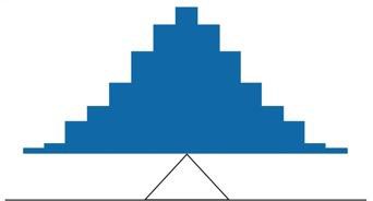
Figure 5. A distribution balanced on the tip of a triangle where the middle point, the median, is also the mean, the point of balance.
More on the Mean and Median
The mean is the point on which a distribution would balance, the median is the value that minimizes the sum of absolute deviations, and the mean is the value that minimizes the sum of the squared deviations. Figure 6 shows the numbers 2, 3, 4, 9, and 16. We calculated the mean as 6.8. The median would be the middle-value number. From the 5 scores, the median is 4.

Figure 6. The distribution balances at the mean of 6.8 and the median of 4.0.
Median
In order to calculate median:
- Arrange the numbers in the set from smallest to largest.
- Determine N or n (number of scores)
- If N or n is odd then the median is the middle number.
- If N or n is even then the median is the average of the middle two numbers
For the data in Table 3 (an example earlier in the chapter with football scores), there are 31 scores. The 16th highest score (which equals 20) is the median because there are 15 scores below the 16th score and 15 scores above the 16th score. Again, the median can also be thought of as the 50th percentile.
When there are numbers with the same values, each appearance of that value gets counted. For example, in the set of numbers 1, 3, 4, 4, 5, 8, and 9, the median is 4 because there are three numbers (1, 3, and 4) below it and three numbers (5, 8, and 9) above it. If we only counted 4 once, the median would incorrectly be calculated at 4.5 (4+5 divided by 2). When in doubt, writing out all of the numbers in order and marking them off one at a time from the top and bottom will always lead you to the correct answer.
Mode
The mode is the most frequently occurring value in the dataset. If there are multiple values “tied” for most frequently occurring, the data set can have more than one mode. If all the values occur at the same rate, then there is no mode.
Mode
In order to find the mode, create a frequency table. Identify the score with the highest frequency. It is the score and not the frequency value that is the mode.
Example: 2,3,4,9,16
There is no mode as each score only has a frequency of 1.
Example: 11, 12, 12, 13, 14
| score | f |
| 11 | 1 |
| 12 | 2 |
| 13 | 1 |
| 14 | 1 |
The mode is 12.
For the data in Table 3, the mode is 18 since more teams (4) had 18 touchdown passes than any other number of touchdown passes. With continuous data, such as response time measured to many decimals, the frequency of each value is one since no two scores will be exactly the same (see discussion of continuous variables). Therefore the mode of continuous data is normally computed from a grouped frequency distribution. Table 2 shows a grouped frequency distribution for the target response time data. Since the interval with the highest frequency is 600-700, the mode is the middle of that interval (650). Though the mode is not frequently used for continuous data, it is nevertheless an important measure of central tendency as it is the only measure we can use on qualitative or categorical data.
|
Range |
Frequency |
|
500-600 600-700 700-800 800-900 900-1000 1000-1100 |
3 6 5 5 0 1 |
Table 5. Grouped frequency distribution
Recap
All measures of central tendency reflect something about the middle of a distribution; but each of the three most common measures of central tendency represents a different concept:
Mean: average, where μ is for the population and 𝑋̅ or M is for the sample (both same equation).
Median: middle or 50th percentile. If N or n is odd then the median is the middle number. If N or n is even then the median is the average of the middle two numbers
Mode: most common, or most frequent value, where there can be a tie or there can be no mode.
Comparing Measures of Central Tendency
A distribution is a graph that shows how scores are distributed along a measurement scale. The mean is the point on the x-axis that falls directly at the “balancing point” for the distribution. The median is the point on the x-axis at which half the area under the distribution curve lies below the median and half lies above the median. The mode is the point on the x-axis that falls directly below the tallest point on the distribution.
In a perfectly symmetrical (normal) distribution, all three measures of central tendency are located at the same value. A distribution is symmetrical if a vertical line can be drawn at some point in the histogram such that the shape to the left and the right of the vertical line are mirror images of each other. In a perfectly symmetrical distribution, the mean and the median are the same. This example has one mode (unimodal), and the mode is the same as the mean and median.How do the various measures of central tendency compare with each other? In a symmetrical distribution that has two modes (bimodal), the two modes would be different from the mean and median.
A skewed distribution has one side that is long and spread out, somewhat like a tail. The side with the fewer scores (the side that looks more like a tail) is considered the direction of the skew. A distribution that is skewed to the right is called a positive skewed. A distribution skewed to the left is called a negative skew.
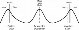
Figure 7. Distributions with mean, median and mode
Differences among the measures occur with skewed distributions. Figure 8 shows the distribution of 642 scores on an introductory psychology test. Notice this distribution has a slight positive skew.
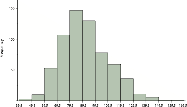
Figure 8. A distribution with a positive skew.
Measures of central tendency are shown in Table 6. Notice they do not differ greatly, with the exception that the mode is considerably lower than the other measures. When distributions have a positive skew, the mean is typically higher than the median, although it may not be in bimodal distributions. For these data, the mean of 91.58 is higher than the median of 90. This pattern holds true for any skew: the mode will remain at the highest point in the distribution, the median will be pulled slightly out into the skewed tail (the longer end of the distribution), and the mean will be pulled the farthest out. Thus, the mean is more sensitive to skew than the median or mode, and in cases of extreme skew, the mean may no longer be appropriate to use.
|
Measure |
Value |
|
Mode Median Mean |
84
90 91.58 |
Table 6. Measures of central tendency for the test scores.
The distribution of baseball salaries (in 1994) shown in Figure 9 has a much more pronounced skew than the distribution in Figure 8.
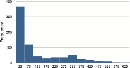
Figure 9. A distribution with a very large positive skew. This histogram shows the salaries of major league baseball players (in thousands of dollars).
Table 7 shows the measures of central tendency for these data. The large skew results in very different values for these measures. No single measure of central tendency is sufficient for data such as these. If you were asked the very general question: “So, what do baseball players make?” and answered with the mean of $1,183,000, you would not have told the whole story since only about one-third of baseball players make that much. If you answered with the mode of $250,000 or the median of $500,000, you would not be giving any indication that some players make many millions of dollars. Fortunately, there is no need to summarize a distribution with a single number. When the various measures differ, our opinion is that you should report the mean and median. Sometimes it is worth reporting the mode as well. In the media, the median is usually reported to summarize the center of skewed distributions. You will hear about median salaries and median prices of houses sold, etc. This is better than reporting only the mean, but it would be informative to hear more statistics.
|
Measure |
Value (in thousands) |
|
Mode Median Mean |
250 500 1,183 |
Summary
Remember that measures of central tendency summarize and organize large sets of data that allow researchers to communicate information with just a few numbers. There are three main considerations when determining which measure of central tendency to use:
| Type | Appropriate | Not Appropriate |
| Mean | Interval/Ratio | Extreme scores
Skewed distribution Ordinal Nominal |
| Median | Extreme scores
Skewed distribution Ordinal |
Nominal |
| Mode | Nominal
Discrete Describe shape – bimodal |
Interval/Ratio |
Before deciding to report a mean, median or mode ask yourself what the data are trying to convey, what is the shape of the distribution (e.g., normal or skewed) and the level of measurement for the data.
The level of measurement of a particular variable will determine which measure(s) of central tendency can be used. For example:
- Mean is preferred when using ratio level data unless distribution includes outliers
- Median is the preferred when using ordinal data
- Median is preferred when data include outliers
- Mode is preferred when using nominal data
The goal of descriptive statistics is to summarize and organize large amounts of data and measures of central tendency tell us about the middle of a distribution but we need to select the measure that is most representative of the distribution.
Generally, if the distribution of data is skewed to the left, the mean is less than the median, which is often less than the mode. If the distribution of data is skewed to the right, the mode is often less than the median, which is less than the mean. The mean will inaccurately describe a skewed (non-symmetrical) distribution. You have seen this happen if you’ve ever received one very low grade in a class after receiving many high grades; your average drops like a rock. The one low grade produces a negatively skewed distribution, and the mean gets pulled away from where most of your grades are, toward that low grade. What hurts is then telling someone your average because it’s misleading. It gives the impression that all of your grades are relatively low, even though you have only that one F.
Learning Objectives
Having read this chapter, you should be able to:
- explain the purpose of measuring central tendency
- define and compute the three measures of central tendency (mean, median, mode)
- list the circumstances where each of the three measures of central tendency are appropriate
- explain how the three measures of central tendency are related to distribution (positive skew, negative skew, normal)
Exercises – Ch. 4
- If the mean time to respond to a stimulus is much higher than the median time to respond, what can you say about the shape of the distribution of response times?
- Compare the mean, median, and mode in terms of their sensitivity to extreme scores.
- Your younger brother comes home one day after taking a science test. He says that some- one at school told him that “60% of the students in the class scored above the median test grade.” What is wrong with this statement? What if he had said “60% of the students scored above the mean?”
- Make up three data sets with 5 numbers each that have:
- the same mean but different standard deviations.
- the same mean but different medians.
- the same median but different means.
- Compute the population mean for the following scores: 5, 7, 8, 3, 4, 4, 2, 7, 1, 6
- Compute the sample mean for the following scores: -8, -4, -7, -6, -8, -5, -7, -9, -2, 0
- For the following problem, use the following scores: 5, 8, 8, 8, 7, 8, 9, 12, 8, 9, 8, 10, 7, 9, 7, 6, 9, 10, 11, 8
- Create a histogram of these data. What is the shape of this histogram?
- How do you think the three measures of central tendency will compare to each other in this dataset?
- Compute the sample mean, the median, and the mode
- Draw and label lines on your histogram for each of the above values. Do your results match your predictions?
Answers to Odd-Numbered Exercises – Ch. 4
1. If the mean is higher, that means it is farther out into the right-hand tail of the distribution. Therefore, we know this distribution is positively skewed. Review Figure 7.
3. The median is defined as the value with 50% of scores above it and 50% of scores below it; therefore, 60% of score cannot fall above the median. If 60% of scores fall above the mean, that would indicate that the mean has been pulled down below the value of the median, which means that the distribution is negatively skewed
5. μ = 4.80
7. M = -6.6
