
12 Chapter 12: Repeated Measures t-test
A new t-test for a different research design
So far, we have dealt with data measured on a single variable at a single point in time, allowing us to gain an understanding of the logic and process behind statistics and hypothesis testing. Now, we will look at a slightly different type of data that has new information we couldn’t get at before: change. Specifically, we will look at how the value of a variable, within people, changes across two time points. This is known as a repeated measures design where the same individual is tested more than once to examine for individual differences. This is a very powerful thing to do, and, as we will see shortly, it involves only a very slight addition to our existing process and does not change the mechanics of hypothesis testing or formulas at all!
Change and Differences
Researchers are often interested in change over time. Sometimes we want to see if change occurs naturally, and other times we are hoping for change in response to some manipulation. In each of these cases, we measure a single variable at different times, and what we are looking for is whether or not we get the same score at time 2 as we did at time 1. This is a repeated sample research design, where a single group of individuals is obtained and each individual is measured in two treatment conditions that are then compared. Data consist of two scores for each individual. This means that all subjects participate in each treatment condition. Think about it like a pretest/posttest or a before-after comparison.
When we analyze data for a repeated research design, we calculate the difference between members of each pair of scores and then take the average of those differences. The absolute value of our measurements does not matter – all that matters is the change. If the average difference between scores in our sample is very large, compared to the difference between scores we would expect if the member was selected from the same population then we will conclude that the individuals were selected from different populations.
Let’s look at an example:
|
Before |
After |
Improvement |
|
6 |
9 |
3 |
|
7 |
7 |
0 |
|
4 |
10 |
6 |
|
1 |
3 |
2 |
|
8 |
10 |
2 |
Table 1. Raw and difference scores before and after training.
The difference score formula
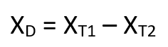
Note: T2 is the time 2 variable; T1 is the time 1 variable
A special case of repeated measures design
We can also test to see if people who are matched or paired in some way agree on a specific topic. We call this a matched design. For example, we can see if a parent and a child agree on the quality of home life, or we can see if two romantic partners agree on how serious and committed their relationship is. In these situations, we also subtract one score from the other to get a difference score. This time, however, it doesn’t matter which score we subtract from the other because what we are concerned with is the agreement.
For repeated measures design (including matched design), what we have are multiple scores on a single variable. That is, a single observation or data point is comprised of two measurements that are put together into one difference score. This is what makes the analysis of change unique – our ability to link these measurements in a meaningful way. This type of analysis would not work if we had two separate samples of people that weren’t related at the individual level, such as samples of people from different states that we gathered independently. Such datasets and analyses are the subject of the following chapter.

We are still working with t-tests. In chapter 11, we compared a sample to a population mean. For t-tests in this chapter, we are comparing 2 groups of scores, yet both are from the same individuals.
2 cups of tea for me: for a repeated measures design the same individuals are in both conditions for a t-test. Photo credit
We call this a dependent t-test or a paired t-test. Sometimes it is also called “paired samples”, “repeated measures”, “dependent measures”, and “dependent samples.”
What all of these names have in common is that they describe the analysis of two scores that are related in a systematic way within people or within pairs, which is what each of the datasets usable in this analysis have in common. Think of it like each person is having 2 cups of tea (or each person has a pair of shoes – two shoes). As such, all of these names are equally appropriate, and the choice of which one to use comes down to preference. In this text, we will refer to paired or dependent samples, though the appearance of any of the other names throughout this chapter should not be taken to refer to a different analysis: they are all the same thing.
Now that we have an understanding of what difference scores are and know how to calculate them, we can use them to test hypotheses. As we will see, this works exactly the same way as testing hypotheses about one sample mean with a t- statistic. The only difference is in the format of the null and alternative hypotheses, where for focus on the difference score.
Hypotheses of Change and Differences for step 1
When we work with difference scores, our research questions have to do with change. Did scores improve? Did symptoms get better? Did prevalence go up or down? Our hypotheses will reflect this. Remember that the null hypothesis is the idea that there is nothing interesting, notable, or impactful represented in our dataset. In a paired samples t-test, that takes the form of ‘no change’. There is no improvement in scores or decrease in symptoms.
- Thus, our null hypothesis is: H0: There is no change or difference H0: μD = 0
- HA: There is a change or difference HA: μD ≠ 0 (2 tail test/non-directional hypothesis)
- HA: The average score increases HA: μD > 0 (1 tail test/directional hypothesis; expected increase)
- HA: The average score decreases HA: μD < 0 (1 tail test/directional hypothesis; expected decrease)
Choosing 1-tail vs 2-tail test
How do you choose whether to use a one-tailed versus a two-tailed test? The two-tailed test is always going to be more conservative, so it’s always a good bet to use that one, unless you had a very strong prior reason for using a one-tailed test. In that case, you should have written down the hypothesis before you ever looked at the data. In Chapter 19, we will discuss the idea of pre-registration of hypotheses, which formalizes the idea of writing down your hypotheses before you ever see the actual data. You should never make a decision about how to perform a hypothesis test once you have looked at the data, as this can introduce serious bias into the results.
We do have to make one main assumption when we use the randomization test, which we refer to as exchangeability. This means that all of the observations are distributed in the same way, such that we can interchange them without changing the overall distribution. The main place where this can break down is when there are related observations in the data; for example, if we had data from individuals in 4 different families, then we couldn’t assume that individuals were exchangeable, because siblings would be closer to each other than they are to individuals from other families. In general, if the data were obtained by random sampling, then the assumption of exchangeability should hold.
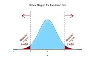
Critical Values and Decision Criteria for step 2
As with before, once we have our hypotheses laid out, we need to find our critical values that will serve as our decision criteria. This step has not changed at all from the last chapter. Our critical values are based on our level of significance (still usually α = 0.05), the directionality of our test (one-tailed or two-tailed), and the degrees of freedom, which are still calculated as df = n – 1. Because this is a t-test like the last chapter, we will find our critical values on the same t-table using the same process of identifying the correct column based on our significance level and directionality and the correct row based on our degrees of freedom or the next lowest value if our exact degrees of freedom are not presented. After we calculate our test statistic, our decision criteria are the same as well: p < α or tobt > tcrit*.
There are a few website options for finding the critical value for p. Here are a few:
- https://www.statology.org/t-score-p-value-calculator/
- https://www.socscistatistics.com/pvalues/tdistribution.aspx
Remember to identify your df (n-1), alpha value, 1 or 2-tail test, and draw the distribution.
Test Statistic for step 3
Our test statistic for our change scores follows exactly the same format as it did for our 1-sample t-test. In fact, the only difference is in the data that we use. For our change test, we first calculate a difference score as shown above. Then, we use those scores as the raw data in the same mean calculation, standard error formula, and t-statistic. Let’s look at each of these.
Mean Difference (top of t-formula) 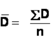 which can also be noted as
  The mean difference score is calculated in the same way as any other mean: sum each of the individual difference scores and divide by the sample size.
Here we are using the subscript D to keep track of that fact that these are difference scores instead of raw scores; it has no actual effect on our calculation.
Using this, we calculate the standard deviation of the difference scores the same way as well:
Standard deviation for D (SD) and variance for D is sD2 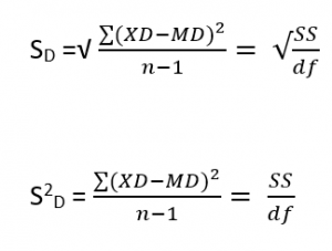 or may see SD noted as
 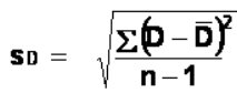 where xD = D & D̅ = MD Note: sD2 = sD * sD and sD = √sD2
We will find the numerator, the Sum of Squares, using the same table format that we learned in chapter 3. Once we have our standard deviation, we can find the standard error:
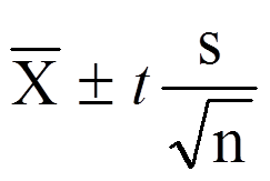
Standard Error Standard error of the mean differences (SMD) (bottom of t-formula): 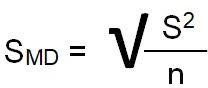 which can also be noted as
 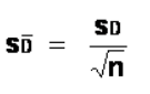 Note: the formula can also be noted as SMD or SD̅ and you can calculate it from the variance (√(s2/n)) or standard deviation( s/√n)
Finally, our test statistic t has the same structure as well:
t-test for paired samples: 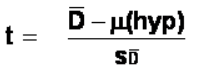 where μ(hyp) is expected to be 0 and is dropped from the calculation formula leaving
 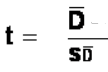 or
or  Note: Both formulas are the same with the mean noted as MD or D̅ and the estimated standard error notes as SMD or SD
 Note: MD is the mean of the difference scores. Reminder we use the same interpretation ranges presented in chapter 10.
| d | Interpretation |
|---|---|
| 0.0 – 0.2 | negligible |
| 0.2 – 0.5 | small |
| 0.5 – 0.8 | medium |
| 0.8 – | large |
Table 2. Interpretation of Cohen’s d
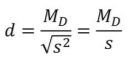
Another way to examine effect size is to report the explained variance for the treatment effect, in other words the percentage of variance accounted for the treatment. This is known as r2. 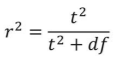 Note: r2 is calculated when there is a reported effect (in other words, null is rejected). Df is the same df from step 2.
As we can see, once we calculate our difference scores from our raw measurements, everything else is exactly the same. Let’s see an example.
Example: Increasing Satisfaction at Work
 Plugging in the values we get 2.85/(√49) = 2.85/7= 0.41 = 2.96/0.41 = 7.22 where the MD or D̅ = 2.96 and a standard deviation of s = 2.85. Plugging in the values we get d=2.96/2.85=1.04 which is a large effect size. We could also calculate r2 for effect size. where t2 = 7.22*7.22 = 52.13 and df = 48. Then plugging in, r2 = 52.13/(52.13+48) = .52. This can be interpreted as 52% of the variance in worker job satisfaction is due to changes the company made.
Hopefully the above example made it clear that running a dependent samples t-test to look for differences before and after some treatment works exactly the same way as a regular 1-sample t-test does from chapter 11 (which was just a small change in how z-tests were performed in chapter 10). At this point, this process should feel familiar, and we will continue to make small adjustments to this familiar process as we encounter new types of data to test new types of research questions.
 but now the mean is the mean difference ( D̅ or MD) and s/√n becomes sD̅ Our adjusted CI formula for paired or dependent t-test: CI = D̅ ± t(sD̅ ) Note: We still calculate an upper bound and lower bound value and t is still the critical value t. CI formula is very similar using the notations for standard error. CI still notated as CI = (LB, UB).
Example with Confidence Interval Hypothesis Testing: Bad Press
Let’s say that a bank wants to make sure that their new commercial will make them look good to the public, so they recruit 7 people to view the commercial as a focus group. The focus group members fill out a short questionnaire about how they view the company, then watch the commercial and fill out the same questionnaire a second time. The bank really wants to find significant results, so they test for a change at α = 0.05. However, they use a 2-tailed test since they know that past commercials have not gone over well with the public, and they want to make sure the new one does not backfire. They decide to test their hypothesis using a confidence interval to see just how spread out the opinions are. As we will see, confidence intervals work the same way as they did before, just like with the test statistic.
Step 1: State the Hypotheses
As always, we start with hypotheses, and with confidence interval hypothesis test, we must use a 2-tail test.
H0: There is no change in how people view the bank H0: μD = 0
HA: There is a change in how people view the bank HA: μD ≠ 0
Step 2: Find the Critical Values
Just like with our regular hypothesis testing procedure, we will need critical values from the appropriate level of significance and degrees of freedom in order to form our confidence interval. Because we have 7 participants, our degrees of freedom are df = 6. From our t-table, we find that the critical value corresponding to this df at this level of significance is t* = 2.447.
Step 3: Calculate the Confidence Interval
The data collected before (time 1) and after (time 2) the participants viewed the commercial is presented in Table 1. In order to build our confidence interval, we will first have to calculate the mean and standard deviation of the difference scores, which are also in Table 1. As a reminder, the difference scores (D̅ or MD) are calculated as Time 2 – Time 1.
|
Time 1 |
Time 2 |
D̅ |
|
3 |
2 |
-1 |
|
3 |
6 |
3 |
|
5 |
3 |
-2 |
|
8 |
4 |
-4 |
|
3 |
9 |
6 |
|
1 |
2 |
1 |
|
4 |
5 |
1 |
Table 3. Opinions of the bank
The mean of the difference scores is: D̅ = 4/7 = .57
The standard deviation will be solved by first using the Sum of Squares Table:
|
D |
D –D̅ |
(D –D̅)2 |
| -1 |
-1.57 |
2.46 |
| 3 |
2.43 |
5.90 |
| -2 |
-2.57 |
6.60 |
| -4 |
-4.57 |
20.88 |
| 6 |
5.43 |
29.48 |
| 1 |
0.43 |
0.18 |
| 1 |
0.43 |
0.18 |
|
Σ = 4 |
Σ = 0 |
Σ = 65.68 (our SS) |
Table 4. Sum of Squared Deviations (SS) calculation for bad press data
s = √SS/df where SS = 65.68 and df = n-1 = 7-1 = 6
Step 4: Make the Decision
Remember that the confidence interval represents a range of values that seem plausible or reasonable based on our observed data. The interval spans -1.86 to 3.00, which includes 0, our null hypothesis value. Because the null hypothesis value is in the interval, it is considered a reasonable value, and because it is a reasonable value, we have no evidence against it. We fail to reject the null hypothesis.
Step 5: Effect size (Cohen’s d or r2)
One option for effect size is Cohen’s d. Performing Cohen’s d = D̅/s = .57/3.308 = .17 which indicates a possible Type II error (very small sample size). As with before, we only report the confidence interval to indicate how we performed the test.
Assumptions of paired t-test
Assumptions are conditions that must be met in order for our hypothesis testing conclusion to be valid. [Important: If the assumptions are not met then our hypothesis testing conclusion is not likely to be valid. Testing errors can still occur even if the assumptions for the test are met.]
Recall that inferential statistics allow us to make inferences (decisions, estimates, predictions) about a population based on data collected from a sample. Recall also that an inference about a population is true only if the sample studied is representative of the population. A statement about a population based on a biased sample is not likely to be true.
Assumption 1: Individuals in the sample were selected randomly and independently, so the sample is highly likely to be representative of the larger population.
• Random sampling ensures that each member of the population is equally likely to be selected.
• An independent sample is one which the selection of one member has no effect on the selection of any other.
Assumption 2: The distribution of sample differences (DSD) is a normal, because we drew the samples from a population that was normally distributed.
- This assumption is very important because we are estimating probabilities using the t- table – which provide accurate estimates of probabilities for events distributed normally.
Assumption 3: Sampled populations have equal variances or have homogeneity of variance.
Advantages & Disadvantages of using a repeated measures design
Advantages. Repeated measure designs reduce the probability of Type I errors when compared with independent sample designs because repeated measure t-tests reduce the probability that we will get a statistically significant difference that is due to an extraneous variable that differed between groups by chance (due to some other factor than the one in which we are interested).
Repeated measure designs are also more powerful (sensitive) than independent sample designs because two scores from each person are compared so each person serves as his or her own control group (we analyze the difference between scores). Repeated measures help identify individual differences.
Disadvantages. Repeated measure t-tests are very sensitive to outside influences and treatment influences. Outside Influences refers to factors outside of the experiment that may interfere with testing an individual across treatment/trials. Examples include mood or health or motivation of the individual participants. Think about it, if a participant tries really hard during the pretest but does not try very hard during the posttest, these differences can create problems later when analyzing the data.
Treatment Influences refers to the events that happen within the testing experience that interferes with how the data are collected. Three of the most common treatment influences are:
1. Practice effect is present where participants perform a task better in later conditions because they have had a chance to practice it.
2. Fatigue effect, where participants perform a task worse in later conditions because they become tired or bored.
3. Order effects refer to differences in research participants’ responses that result from the order (e.g., first, second, third) in which the experimental materials are presented to them.
Imagine, for example, that participants judge the guilt of an attractive defendant and then judge the guilt of an unattractive defendant. If they judge the unattractive defendant more harshly, this might be because of his unattractiveness. But it could be instead that they judge him more harshly because they are becoming bored or tired. In other words, the order of the conditions is a confounding variable. The attractive condition is always the first condition and the unattractive condition the second. Thus any difference between the conditions in terms of the dependent variable could be caused by the order of the conditions and not the independent variable itself.
There is a solution to the problem of order effects, however, that can be used in many situations. It is counterbalancing, which means testing different participants in different orders. For example, some participants would be tested in the attractive defendant condition followed by the unattractive defendant condition, and others would be tested in the unattractive condition followed by the attractive condition. With three conditions, there would be six different orders (ABC, ACB, BAC, BCA, CAB, and CBA), so some participants would be tested in each of the six orders. With counterbalancing, participants are assigned to orders randomly, using the techniques we have already discussed. Thus random assignment plays an important role in within-subjects designs just as in between-subjects designs. Here, instead of randomly assigning to conditions, they are randomly assigned to different orders of conditions. In fact, it can safely be said that if a study does not involve random assignment in one form or another, it is not an experiment.
Because the repeated-measures design requires that each individual participate in more than one treatment, there is always the risk that exposure to the first treatment will cause a change in the participants that influences their scores in the second treatment that have nothing to do with the intervention. For example, if students are given the same test before and after the intervention the change in the posttest might be because the student got practice taking the test, not because the intervention was successful.
Learning Objectives
Having read this chapter, a student should be able to:
- identify when appropriate to calculate a paired or dependent t-test
- perform a hypothesis test using the paired or dependent t-test
- compute and interpret effect size for dependent or paired t-test
- list the assumptions for running a paired or dependent t-test
- list the advantages and disadvantages for a repeated measures design
Exercises – Ch. 12
- What is the difference between a 1-sample t-test and a dependent-samples t– test? How are they alike?
- Name 3 research questions that could be addressed using a dependent- samples t-test.
- What are difference scores and why do we calculate them?
- Why is the null hypothesis for a dependent-samples t-test always μD = 0?
- A researcher is interested in testing whether explaining the processes of statistics helps increase trust in computer algorithms. He wants to test for a difference at the α = 0.05 level and knows that some people may trust the algorithms less after the training, so he uses a two-tailed test. He gathers pre- post data from 35 people and finds that the average difference score is 12.10 with a standard deviation (s) is 17.39. Conduct a hypothesis test to answer the research question.
- Decide whether you would reject or fail to reject the null hypothesis in the following situations:
- M𝐷̅ = 3.50, s = 1.10, n = 12, α = 0.05, two-tailed test
- 95% CI = (0.20, 1.85)
- t = 2.98, t* = -2.36, one-tailed test to the left
- 90% CI = (-1.12, 4.36)
- Calculate difference scores for the following data:
|
Time 1 |
Time 2 |
XD or D |
|
61 |
83 |
|
|
75 |
89 |
|
|
91 |
98 |
|
|
83 |
92 |
|
|
74 |
80 |
|
|
82 |
88 |
|
|
98 |
98 |
|
|
82 |
77 |
|
|
69 |
88 |
|
|
76 |
79 |
|
|
91 |
91 |
|
|
70 |
80 |
|
8. You want to know if an employee’s opinion about an organization is the same as the opinion of that employee’s boss. You collect data from 18 employee-supervisor pairs and code the difference scores so that positive scores indicate that the employee has a higher opinion and negative scores indicate that the boss has a higher opinion (meaning that difference scores of 0 indicate no difference and complete agreement). You find that the mean difference score is ̅𝑋̅̅𝐷̅ = -3.15 with a standard deviation of sD = 1.97. Test this hypothesis at the α = 0.01 level.
9. Construct confidence intervals from a mean = 1.25, standard error of 0.45, and df = 10 at the 90%, 95%, and 99% confidence level. Describe what happens as confidence changes and whether to reject H0.
10.A professor wants to see how much students learn over the course of a semester. A pre-test is given before the class begins to see what students know ahead of time, and the same test is given at the end of the semester to see what students know at the end. The data are below. Test for an improvement at the α = 0.05 level. Did scores increase? How much did scores increase?
|
Pretest |
Posttest |
XD |
|
90 |
8 |
|
|
60 |
66 |
|
|
95 |
99 |
|
|
93 |
91 |
|
|
95 |
100 |
|
|
67 |
64 |
|
|
89 |
91 |
|
|
90 |
95 |
|
|
94 |
95 |
|
|
83 |
89 |
|
|
75 |
82 |
|
|
87 |
92 |
|
|
82 |
83 |
|
|
82 |
85 |
|
|
88 |
93 |
|
|
66 |
69 |
|
|
90 |
90 |
|
|
93 |
100 |
|
|
86 |
95 |
|
|
91 |
96 |
|
Answers to Odd- Numbered Exercises – Ch. 12
1. A 1-sample t-test uses raw scores to compare an average to a specific value. A dependent samples t-test uses two raw scores from each person to calculate difference scores and test for an average difference score that is equal to zero. The calculations, steps, and interpretation is exactly the same for each.
7. See table last column.
|
Time 1 |
Time 2 |
D or XD |
|
61 |
83 |
22 |
|
75 |
89 |
14 |
|
91 |
98 |
7 |
|
83 |
92 |
9 |
|
74 |
80 |
6 |
|
82 |
88 |
6 |
|
98 |
98 |
0 |
|
82 |
77 |
-5 |
|
69 |
88 |
19 |
|
76 |
79 |
3 |
|
91 |
91 |
0 |
|
70 |
80 |
10 |
9. At the 90% confidence level, t* = 1.812 and CI = (0.43, 2.07) so we reject H0. At the 95% confidence level, t* = 2.228 and CI = (0.25, 2.25) so we reject H0. At the 99% confidence level, t* = 3.169 and CI = (-0.18, 2.68) so we fail to reject H0. As the confidence level goes up, our interval gets wider (which is why we have higher confidence), and eventually we do not reject the null hypothesis because the interval is so wide that it contains 0.
