Chapter 11: Introduction to t-tests

Alisa Beyer

11 Chapter 11: Introduction to t-tests

In this unit, we made a big leap from basic descriptive statistics into full hypothesis testing and inferential statistics. For the rest of the unit, we will be learning new tests, each of which is just a small adjustment on the test before it. In this chapter, we will learn about the first of three t-tests, and we will learn a new method of testing the null hypothesis: confidence intervals.

At this point, we may think we know all about hypothesis testing. Here’s a surprise – what we know will not help you much as a researcher. Why? The procedures for testing hypotheses described up to this point were, of course, absolutely necessary for what comes next, but these procedures involved comparing a group of scores to a known population. In real research practice, we often compare two or more groups of scores to each other, without any direct information about populations. For example:

Comparing the intelligence scores (IQ) of one sample to standardized IQ norms and population values.
Comparing pre and post-test anxiety scores for a group of patients before and after psychotherapy or number of familiar versus unfamiliar words recalled in a memory experiment.
Comparing scores on a cognitive test for a group of participants experiencing sleep deprivation and a group of participants who slept normally.
Comparing scores on self-esteem test scores for a group of 10-year-old girls to a group of 10-year-old boys.

These kinds of research situations are among the most common in psychology, where the only information available is usually from samples. Nothing is known about the populations that the samples are supposed to come from. In particular, the researcher does not know the variance of the populations involved. In this chapter, we will learn the solution to the problem of the unknown population variance.

The hypothesis-testing procedures we learn in this chapter (and a few others) are examples of t-tests. Its main principles were originally developed by William S. Gosset who published his research articles anonymously using the name “Student”.

William S. Gosset graduated from Oxford University in 1899 with degrees in mathematics and chemistry. It happened that in the same year the Guinness brewers in Dublin, Ireland, were seeking a few young scientists to take a first-ever scientific look at beer making. Gosset took one of these jobs and soon had immersed himself in barley, hops, and vats of brew.

Photo in the public domain.

The problem was how to make a beer of consistently high quality. Scientists want to make a quality beer less variable, and were especially interested in finding the cause of bad batches. But a business such as a brewery could not afford to waste money on experiments involving large numbers of vats. So, Gosset was forced to contemplate the probability of a certain strain of barley producing terrible beer when the experiment could consist of only a few batches of each strain. So, from this Gosset discovered the t distribution and invented the t-test.

Most of his work was done on the back of envelopes, with plenty of minor errors in arithmetic that had to be worked out later. He published his paper on his “brewery methods” only when editors of scientific journals demanded. At that time, the Guinness brewery did not allow a scientist to publish papers, because more than one Guinness scientist has revealed brewery secrets. To this day, most scientists call the t- distribution “Student’s t” because Gosset wrote under the anonymous name “Student” so that the brewery would not know about his writing or be identified through his being known to be its employee. Supposedly, the brewery learned of his scientific fame only at his death, when colleagues wanted to honor him.

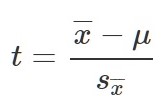
The t-statistic for one-sample (compared to population mean)

Last chapter, we were introduced to hypothesis testing using the z-statistic for sample means that we learned in Unit 1. This was a useful way to link the material and ease us into the new way to looking at data, but it isn’t a very common test because it relies on knowing the population standard deviation, σ, which is rarely going to be the case. Instead, we will estimate that parameter σ using the sample statistics in the same way that we estimate μ using ̅X (μ will still appear in our formulas because we suspect something about its value and that is what we are testing). Our new statistic is called t, and for testing one population mean using a single sample (called a 1-sample t-test) it takes the form:

1-sample t-test:

t is mean differences over the estimated standard error

in other words

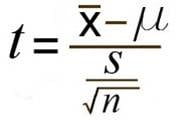
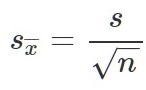
Notice that t looks almost identical to z; this is because they test the exact same thing: the value of a sample mean compared to what we expect of the population. The only difference is that the standard error is now denoted 𝑠_X̅ or s_Mto indicate that we use the sample statistic for standard deviation, s, instead of the population parameter σ. We call the standard error using s, the estimated standard error of the mean. The process of using and interpreting the standard error and the full test statistic remain exactly the same.

Estimated standard error of the mean 𝑠_X̅ or s_M

or equivalent

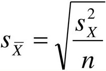
Note: Formulas can notate as 𝑠_X̅ or s_M.You can calculate estimated standard error using the sample standard deviation (s) or sample variance (s₂).

Setting up for step 2

In order to find the critical boundary for a t-test we must use degrees of freedom. In chapter 4 we learned that the formulae for sample standard deviation and population standard deviation differ by one key factor: the denominator for the parameter is N but the denominator for the statistic is n – 1, also known as degrees of freedom, df. As we learned earlier, degrees of freedom gets its name because it is the number of scores in a sample that are “free to very”. The idea is that when finding the variance we must first know the mean. If we know the mean and all but one of the scores in a sample, we can figure out the one we do not know with a little math. In this situation the degrees of freedom is the number of scores minus 1.

Because we are using a new measure of spread, we can no longer use the standard normal distribution and the z-table to find our critical values. For t-tests, we will use the t-distribution and t-table to find these values.

The t-distribution, like the standard normal distribution, is symmetric and normally distributed with a mean of 0 and standard error (as the measure of standard deviation for sampling distributions) of 1. However, because the calculation of standard error uses degrees of freedom, there will be a different t-distribution for every degree of freedom. Luckily, they all work exactly the same, so in practice this difference is minor.

Figure 1 shows four curves: a normal distribution curve labeled z, and three t– distribution curves for 2, 10, and 30 degrees of freedom. Remember degrees of freedom refers to the maximum number of logically independent values, which are values that have the freedom to vary, in the data sample. Two things should stand out: First, for lower degrees of freedom (e.g., 2), the tails of the distribution are much fatter, meaning a larger proportion of the area under the curve falls in the tail. This means that we will have to go farther out into the tail to cut off the portion corresponding to 5% or α = 0.05, which will, in turn, lead to higher critical (rejection) values. Second, as the degrees of freedom increase, we get closer and closer to the z curve. Even the distribution with df = 30, corresponding to a sample size of just 31 people, is nearly indistinguishable from z. In fact, a t-distribution with infinite degrees of freedom (theoretically, of course) is exactly the standard normal distribution. Because of this, the bottom row of the t-table also includes the critical values for z-tests at the specific significance levels. Even though these curves are very close, it is still important to use the correct table and critical values, because small differences can add up quickly.

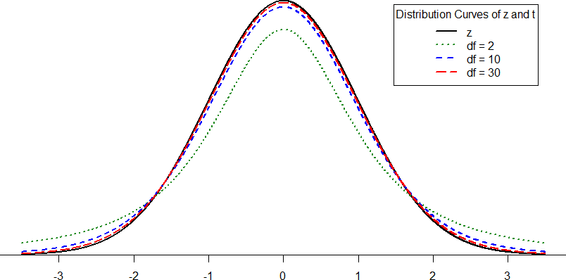
Figure 1. Distributions comparing effects of degrees of freedom

The t-distribution table lists critical values for one- and two-tailed tests at several levels of significance arranged into columns. The rows of the t-table list degrees of freedom up to df = 100 in order to use the appropriate distribution curve. It does not, however, list all possible degrees of freedom in this range, because that would take too many rows. Above df = 40, the rows jump in increments of 10. If a problem requires you to find critical values and the exact degrees of freedom is not listed, you always round down to the next smallest number. For example, if you have 48 people in your sample, the degrees of freedom are n – 1 = 48 – 1 = 47; however, 47 doesn’t appear on our table, so we round down and use the critical values for df = 40, even though 50 is closer. We do this because it avoids inflating Type I Error (false positives, see chapter 9) by using criteria that are too lax.

Hypothesis Testing with t

Hypothesis testing with the t-statistic works exactly the same way as z-tests did, following the four-step process of 1) Stating the Hypothesis, 2) Finding the Critical Values, 3) Computing the Test Statistic, and 4) Making the Decision. Just like the z-statistic, our ultimate goal is to decide whether to reject or fail to reject the null hypothesis.

We will work through an example: let’s say that you move to a new city and find an auto shop to change your oil. Your old mechanic did the job in about 30 minutes (though you never paid close enough attention to know how much that varied), and you suspect that your new shop takes much longer. After 4 oil changes, you think you have enough evidence to demonstrate this.

Step 1: State the Hypotheses

Our hypotheses for 1-sample t-tests are identical to those we used for z-tests. We still state the null and alternative hypotheses mathematically in terms of the population parameter and written out in readable English. In the example, the individual hypothesized that the shop took longer (increased time) which is phrased as a directional research hypothesis, corresponding to a 1-tail test.

For our example:

H₀: There is no difference in the average time to change a car’s oil – mathematically can be phrased as, H₀: μ = 30

H_A: This shop takes longer to change oil than your old mechanic – mathematically can be phrased as, H_A: μ > 30

It is important to set up the hypotheses giving context of the problem/study (using words) and mathematically connecting to the population mean (μ) that is reported in the problem/study (or in real life you would look up or calculate from a given data set).

Step 2: Find the Critical Values

As noted above, our critical values still delineate the area in the tails under the curve corresponding to our chosen level of significance. Because we have no reason to change significance levels, we will use α = 0.05, and because we suspect a direction of effect, we have a one-tailed test. To find our critical values for t, we need to add one more piece of information: the degrees of freedom.

For this example: df = n – 1 = 4 – 1 = 3

Going to our t-table, we find the column corresponding to our one-tailed significance level and find where it intersects with the row for 3 degrees of freedom. As shown in Figure 2: our critical value is t* = 2.353

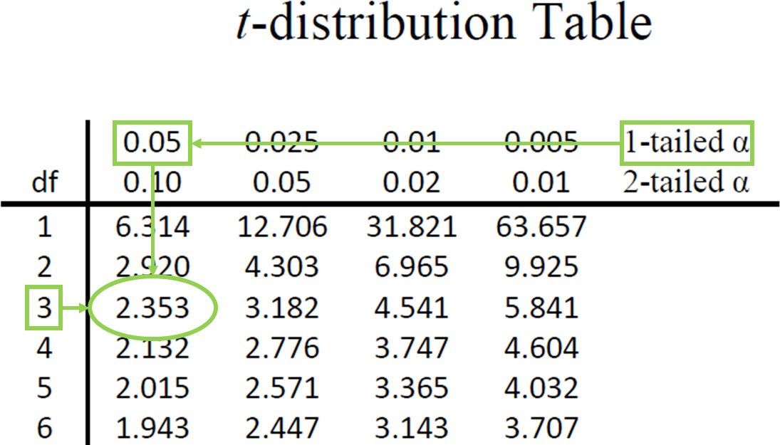
Figure 2. t-table

We can then shade this region on our t-distribution to visualize our critical rejection region

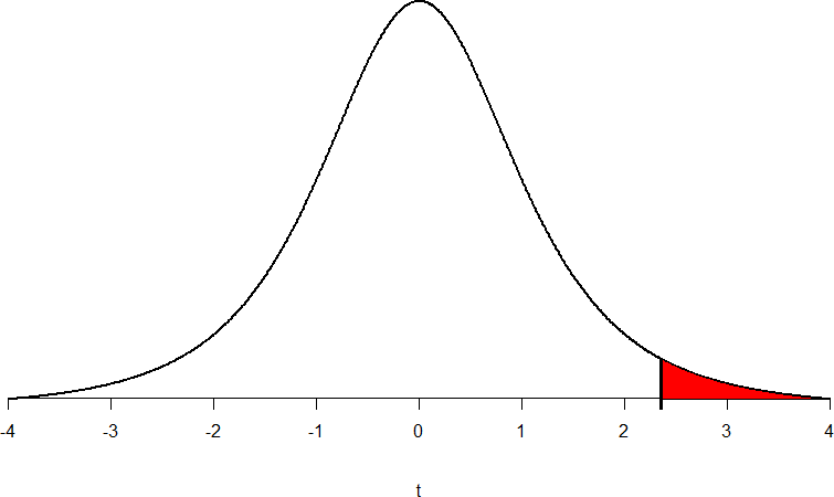
Figure 3. Critical Rejection Region calculated from df and identified using the t-distribution Table.

Step 3: Compute the Test Statistic

The four wait times you experienced for your oil changes are the new shop were 46 minutes, 58 minutes, 40 minutes, and 71 minutes. We will use these to calculate ̅X and s by first filling in the sum of squares table in Table 1:

X	X – ̅X	(X – ̅X)²
46	-7.75	60.06
58	4.25	18.06
40	-13.75	189.06
71	17.25	297.56
Σ = 215	Σ = 0	Σ = 564.74

Table 1. Sum of Squares Table

After filling in the first row to get ΣX = 215, we find that the mean is ̅X = 53.75 (215 divided by sample size 4), which allows us to fill in the rest of the table to get our sum of squares SS = 564.74, which we then plug in to the formula for standard deviation from chapter 3:

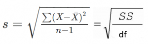
Plugging in SS = 564.74 and df = 3, we get s = 13.72. Next, we take this value and plug it in to the formula for standard error:

Plugging in s = 13.72 and √n = √4 = 2, we get S_̅X=6.86. And, finally, we put the standard error, sample mean, and null hypothesis value into the formula for our test statistic t:

Plugging in ̅X=53.75, μ = 30, and S_̅X=6.86, we get 23.75/6.68 = 3.46. This may seem like a lot of steps, but it is really just taking our raw data to calculate one value at a time and carrying that value forward into the next equation: data → sample size/degrees of freedom → mean → sum of squares → standard deviation → standard error → test statistic. At each step, we simply match the symbols of what we just calculated to where they appear in the next formula to make sure we are plugging in everything correctly. Also, for this class, you may directly given the standard deviation and mean to work from, so be sure to identify where you are starting from if not given the data to work through the entire problem.

Step 4: Make the Decision

Now that we have our critical value and test statistic, we can make our decision using the same criteria we used for a z-test. Our obtained t-statistic was t = 3.46 and our critical value was t* = 2.353: t > t*, so we reject the null hypothesis and conclude:

Based on our four oil changes, the new mechanic takes longer on average (̅X = 53.75) to change oil than our old mechanic, t(3) = 3.46, p < .05.

Notice that we also include the degrees of freedom in parentheses next to t. We need to calculate an effect size, which is still Cohen’s d, but now we use s in place of σ:

Cohen’s d 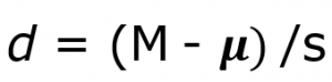Example: d = (53.75-30)/13.72 = 1.73

For this example, d = (53.75-30)/13.72 = 1.73. This is a large effect. It should also be noted that for some things, like the minutes in our current example, we can also interpret the magnitude of the difference we observed (23 minutes and 45 seconds) as an indicator of importance since time is a familiar metric.

Confidence Intervals

Up to this point, we have learned how to estimate the population parameter for the mean using sample data and a sample statistic. From one point of view, this makes sense: we have one value for our parameter so we use a single value (called a point estimate) to estimate it. However, we have seen that all statistics have sampling error and that the value we find for the sample mean will bounce around based on the people in our sample, simply due to random chance. Thinking about estimation from this perspective, it would make more sense to take that error into account rather than relying just on our point estimate. To do this, we calculate what is known as a confidence interval.

A confidence interval starts with our point estimate then creates a range of scores considered plausible based on our standard deviation, our sample size, and the level of confidence with which we would like to estimate the parameter. This range, which extends equally in both directions away from the point estimate, is called the margin of error. We calculate the margin of error by multiplying our two-tailed critical value by our standard error:

Margin of Error (MOE) Margin of Error =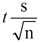

where s = standard deviation and t is the critical value t. The MOE is the t-critical value times the estimated standard error, S_̅X.

One important consideration when calculating the margin of error is that it can only be calculated using the critical value for a two-tailed test. This is because the margin of error moves away from the point estimate in both directions, so a one- tailed value does not make sense.

The critical value we use will be based on a chosen level of confidence, which is equal to 1 – α. Thus, a 95% level of confidence corresponds to α = 0.05. Thus, at the 0.05 level of significance, we create a 95% Confidence Interval. How to interpret that is discussed further on.

Once we have our margin of error calculated, we add it to our point estimate for the mean to get an upper bound to the confidence interval and subtract it from the point estimate for the mean to get a lower bound for the confidence interval:

Confidence Intervals (CI)

CI = 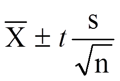where is the Margin of Error (MOE)

You will calculate an upper bound value and a lower bound value.

Upper bound (UB)= use the + in the CI formula = ̅X+MOE

Lower bound (LB) = use the + in the CI formula = ̅X – MOE

To write out a confidence interval, we always use soft brackets and put the lower bound, a comma, and the upper bound:

Confidence Interview = (LB value, UB value)

Let’s see what this looks like with some actual numbers by taking our oil change data and using it to create a 95% confidence interval estimating the average length of time it takes at the new mechanic. We already found that our average was ̅X =53.75 and our standard error was s_𝑋̅ = 6.86.

We also found a critical value to test our hypothesis, but remember that we were testing a one-tailed hypothesis, so that critical value won’t work. To see why that is, look at the column headers on the t– table. The column for one-tailed α = 0.05 is the same as a two-tailed α = 0.10. If we used the old critical value, we’d actually be creating a 90% confidence interval (1.00-0.10 = 0.90, or 90%). To find the correct value, we use the column for two- tailed α = 0.05 and, again, the row for 3 degrees of freedom, to find t* = 3.182.

Now we have all the pieces we need to construct our confidence interval:

95% CI = 53.75 ± 3.182(6.86)

upper bound = 53.75 + 3.182(6.86)

UB = 53.75 + 21.83 = 75.58

lower bound = 53.75 − 3.182(6.86)

LB = 53.75 − 21.83 = 31.92

95% CI = (31.92, 75.58)

So we find that our 95% confidence interval runs from 31.92 minutes to 75.58 minutes, but what does that actually mean? The range (31.92, 75.58) represents values of the mean that we consider reasonable or plausible based on our observed data. It includes our point estimate of the mean, ̅X = 53.75, in the center, but it also has a range of values that could also have been the case based on what we know about how much these scores vary (i.e. our standard error).

It is very tempting to also interpret this interval by saying that we are 95% confident that the true population mean falls within the range (31.92, 75.58), but this is not true. The reason it is not true is that phrasing our interpretation this way suggests that we have firmly established an interval and the population mean does or does not fall into it, suggesting that our interval is firm and the population mean will move around. However, the population mean is an absolute that does not change; it is our interval that will vary from data collection to data collection, even taking into account our standard error. The correct interpretation, then, is that we are 95% confident that the range (31.92, 75.58) brackets the true population mean. This is a very subtle difference, but it is an important one.

Interpreting Confidence Intervals

Confidence intervals are notoriously confusing, primarily because they don’t mean what we might intuitively think they mean. If I tell you that I have computed a “95% confidence interval” for my statistic, then it would seem natural to think that we can have 95% confidence that the true parameter value falls within this interval. However, as we will see throughout the course, concepts in statistics often don’t mean what we think they should mean. In the case of confidence intervals, we can’t interpret them in this way because the population parameter has a fixed value – it either is or isn’t in the interval, so it doesn’t make sense to talk about the probability of that occurring. Jerzy Neyman, the inventor of the confidence interval, said:

“The parameter is an unknown constant and no probability statement concerning its value may be made.”(Neyman 1937)

Instead, we have to view the confidence interval procedure from the same standpoint that we viewed hypothesis testing: As a procedure that in the long run will allow us to make correct statements with a particular probability. Thus, the proper interpretation of the 95% confidence interval is that it is an interval that will contain the true population mean 95% of the time.

Hypothesis Testing with Confidence Intervals

As a function of how they are constructed, we can also use confidence intervals to test hypotheses. However, we are limited to testing two-tailed hypotheses only for this, because of how the intervals work, as discussed above.

Once a confidence interval has been constructed, using it to test a hypothesis is simple.

The range of the confidence interval brackets (or contains, or is around) the null hypothesis value, we fail to reject the null hypothesis.
If it does not bracket the null hypothesis value (i.e. if the entire range is above the null hypothesis value or below it), we reject the null hypothesis.

The reason for this is clear if we think about what a confidence interval represents. Remember: a confidence interval is a range of values that we consider reasonable or plausible based on our data. Thus, if the null hypothesis value is in that range, then it is a value that is plausible based on our observations. If the null hypothesis is plausible, then we have no reason to reject it. Thus, if our confidence interval brackets the null hypothesis value, thereby making it a reasonable or plausible value based on our observed data, then we have no evidence against the null hypothesis and fail to reject it. However, if we build a confidence interval of reasonable values based on our observations and it does not contain the null hypothesis value, then we have no empirical (observed) reason to believe the null hypothesis value and therefore reject the null hypothesis.

Let’s see an example of hypothesis testing using Confidence Intervals

You hear that the national average on a measure of friendliness is 38 points. You want to know if people in your community are more or less friendly than people nationwide, so you collect data from 30 random people in town to look for a difference. We’ll follow the same four-step hypothesis testing procedure as before.

Step 1: State the Hypotheses

We will start by laying out our null and alternative hypotheses:

H₀: There is no difference in how friendly the local community is compared to the national average; H₀: μ = 38

H_A: There is a difference in how friendly the local community is compared to the national average; H_A: μ ≠ 38

Remember we must use a 2-tail test for this, so your hypotheses would be non-directional.

Step 2: Find the Critical Values

We need our critical values in order to determine the width of our margin of error. We will assume a significance level of α = 0.05 (which will give us a 95% CI).

From the t-table, a two-tailed critical value at α = 0.05 with 29 degrees of freedom (n – 1 = 30 – 1 = 29) is t* = 2.045.

Step 3: Calculations

Now we can construct our confidence interval. After we collect our data, we find that the average person in our community scored 39.85, or ̅X= 39.85, and our standard deviation was s = 5.61. First, we need to use this standard deviation, plus our sample size of n = 30, to calculate our standard error:

s_̅X = s/√n = 5.61/√30 = 1.02

Now we can put that value (1.02 as S_̅X), our point estimate for the sample mean (39.85), and our critical t-value from step 2 (2.045) into the formula for a confidence interval:

95% CI= 39.85 ± 2.045(1.02)

UB= 39.85 + 2.045(1.02) = 39.85 + 2.09 = 41.94

LB = 39.85 − 2.045(1.02)= 39.85 − 2.09 = 37.76

95% CI = (37.76, 41.94)

Step 4: Make the Decision

Finally, we can compare our confidence interval to our null hypothesis value. The null value of 38 is higher than our lower bound of 37.76 and lower than our upper bound of 41.94. Thus, the confidence interval brackets our null hypothesis value, and we fail to reject the null hypothesis:

Fail to Reject H₀. Based on our sample of 30 people, our community not different in average friendliness ( ̅X = 39.85) than the nation as a whole, 95% CI = (37.76, 41.94).

Note that we don’t report a test statistic or p-value because that is not how we tested the hypothesis, but we do report the value we found for our confidence interval.

An important characteristic of hypothesis testing is that both methods will always give you the same result. That is because both are based on the standard error and critical values in their calculations. To check this, we can calculate a t-statistic for the example above and find it to be t = 1.81, which is smaller than our critical value of 2.045 and fails to reject the null hypothesis.

Although we failed to reject the null, we can calculate Cohen’s d = ( ̅X – µ)/s = (39.85-38)/5.61 = .33. d = .33 is a small effect size suggesting that we may have a Type II error.

Note: we can also calculate confidence intervals for z. Confidence intervals can also be constructed using z-score criteria, if one knows the population standard deviation. The format, calculations, and interpretation are all exactly the same, only replacing t* with z* and s_̅X with σ_̅X.

Exercises – Ch. 11

What is the difference between a z-test and a 1-sample t-test?
What does a confidence interval represent?
What is the relationship between a chosen level of confidence for a confidence interval and how wide that interval is? For instance, if you move from a 95% CI to a 90% CI, what happens? Hint: look at the t-table to see how critical values change when you change levels of significance.
Construct a confidence interval around the sample mean ̅X = 25 for the following conditions:
1. n = 25, s = 15, 95% confidence level
2. n = 25, s = 15, 90% confidence level
3. _sX̅ = 4.5, α = 0.05, df = 20
4. s = 12, df = 16 (yes, that is all the information you need)
True or False: a confidence interval represents the most likely location of the true population mean.
You hear that college campuses may differ from the general population in terms of political affiliation, and you want to use hypothesis testing to see if this is true and, if so, how big the difference is. You know that the average political affiliation in the nation is μ = 4.00 on a scale of 1.00 to 7.00, so you gather data from 150 college students across the nation to see if there is a difference. You find that the average score is 3.76 with a standard deviation of 1.52. Use a 1-sample t-test to see if there is a difference at the α = 0.05 level.
You hear a lot of talk about increasing global temperature, so you decide to see for yourself if there has been an actual change in recent years. You know that the average land temperature from 1951-1980 was 8.79 degrees Celsius. You find annual average temperature data from 1981-2017 and decide to construct a 99% confidence interval (because you want to be as sure as possible and look for differences in both directions, not just one) using this data to test for a difference from the previous average.
Determine whether you would reject or fail to reject the null hypothesis in the following situations:
1. t = 2.58, N = 21, two-tailed test at α = 0.05
2. t = 1.99, N = 49, one-tailed test at α = 0.01
3. μ = 47.82, 99% CI = (48.71, 49.28)
4. μ = 0, 95% CI = (-0.15, 0.20)
You are curious about how people feel about craft beer, so you gather data from 55 people in the city on whether or not they like it. You code your data so that 0 is neutral, positive scores indicate liking craft beer, and negative scores indicate disliking craft beer. You find that the average opinion was ̅X= 1.10 and the spread was s = 0.40, and you test for a difference from 0 at the α = 0.05 level.
You want to know if college students have more stress in their daily lives than the general population (μ = 12), so you gather data from 25 people to test your hypothesis. Your sample has an average stress score of ̅X = 13.11 and a standard deviation of s = 3.89. Use a 1-sample t-test to see if there is a difference.

Answers to Odd- Numbered Exercises – Ch. 11

1. A z-test uses population standard deviation for calculating standard error and gets critical values based on the standard normal distribution. A t-test uses sample standard deviation as an estimate when calculating standard error and gets critical values from the t-distribution based on degrees of freedom.

3. As the level of confidence gets higher, the interval gets wider. In order to speak with more confidence about having found the population mean, you need to cast a wider net. This happens because critical values for higher confidence levels are larger, which creates a wider margin of error.

5. False: a confidence interval is a range of plausible scores that may or may not bracket the true population mean.

7. ̅X = 9.44, s = 0.35, s_̅X = 0.06, df = 36, t* = 2.719, 99% CI = (9.28, 9.60); CI does not bracket μ, reject null hypothesis. d = 1.83

9. Step 1: H₀: μ = 0 “The average person has a neutral opinion towards craft beer”, H_A: μ ≠ 0 “Overall people will have an opinion about craft beer, either good or bad.”

Step 2: Two-tailed test, df = 54, t* = 2.009.

Step 3: ̅X = 1.10, s_X̅ = 0.05, t = 22.00.

Step 4: t > t*, Reject H₀. Based on opinions from 55 people, we can conclude that the average opinion of craft beer (̅X = 1.10) is positive, t(54) = 22.00, p < .05. Since the result is significant, we need an effect size: Cohen’s d = 2.75, which is a large effect.

License

Icon for the Creative Commons Attribution-NonCommercial-ShareAlike 4.0 International License

Introduction to Statistics for Psychology Copyright © 2021 by Alisa Beyer is licensed under a Creative Commons Attribution-NonCommercial-ShareAlike 4.0 International License, except where otherwise noted.