15 Chapter 15: 2 – Factor ANOVA

A step up for ANOVA

A single factor ANOVA is the statistical analysis appropriate when we are analyzing the results of an experiment in which we have one factor and are looking for differences in the response variable among three or more groups, each of which is receiving different levels or amounts of the factor. In chapter 14, we learned about the single factor ANOVA, also known as the one-way.  We will now conceptually review a multi-factor ANOVA.  We will keep it on the simpler side and use 2-factors (two independent/predictor variables) using a between-subjects design.

Logic of a 2 Factor ANOVA

A two factor ANOVA is used when we believe that more than one factor may affect a particular response (dependent) variable. For example, believe that the age of an adolescent will have an impact on number of phone calls made to the opposite sex and I also suspect that gender of the adolescent will have an impact on the number of phone calls made to the opposite sex.

To test my hypothesis that Age and Biologial Sex of an adolescent will impact the number of phone calls made in the past week. In this case, we have a between-subjects design for both age and biological sex.  I have 2 conditions/levels/groups for each factor/variable. I will have to collect data for these for 4 samples of participants:

Age	Biological sex  (male & female)
	Teen Males	Teen Females
	Older Males	Older Females

Table 1. Example of 2×2 ANOVA

A 2×2 ANOVA gives you 4 conditions.  Note: one way to identify the total conditions in a factorial study is to multiply the conditions for each factor. Thus, a 2×2 design is 2 times 2 giving us 4 total conditions for the study. We will discuss this more in a moment.

Remember that there are different types of ANOVAs based on design.  In this case, we have a between-subjects design.  An individual can only be in 1 condition for gender and 1 condition for age.  So among the 4 total conditions/levels/groups between the 2 factors, an individual is only in 1 of the samples.  For a between-subjects design, there are 4 different samples.  Two Factor ANOVA data is commonly organized like the table above and is referred to a matrix. When the data is organized in a matrix it is very easy to see the factors, as well as the separate levels of the factors.

• Factorial designs like the 2-Factor ANOVA allow a researcher to examine more than one independent variable on the dependent variable
  • Individually for each factor, reporting out a F for each
  • Collectively where the collective influence of the factors is referred to as an interaction. An interaction is the result of the two independent variables combining to produce a result that is different from a result that is produced by either variable alone.

• A 2-Factor ANOVA allows a researcher to assess the main effects (the independent variables) and the interaction yielding three outcomes (3 Fs), a F for factor 1, a F for factor 2 and an interaction between factor 1 and 2.

Let’s go back to our example:

• Main Effect of Factor A
  • Is there a significant effect of age of teen (Factor A) on number of phone calls made to the opposite sex (response variable).

• Main Effect of Factor B
  • Is there a significant effect of sex of the teen (Factor B) on number of phone calls made (response variable).

• Interaction of AxB
  • Does the effect of age of teen (Factor A) on the number of phone calls made (response variable) depend on the sex of the teen (Factor B)?

Conducting a Two Factor ANOVA

Before we begin the process of calculating a 2-Factor ANOVA we need to review several key elements of the study:

• Factors: the independent variables/predictors
• Levels of each factor: how many conditions/groups/treatments a factor has
• Response variable: this is the dependent variable/outcome variable/measurement taken
• Total number of condition in the experiment: this is identified by multiplying out the number of levels for each factor
• Number of subjects per condition, n: how many participants are in each level/group/treatment
• Total number of experiment participants, N: this will be determined by type of factor for each. In a between-group design, there will be four different conditions of participants.  In a complete repeated measures design, all participants are in all conditions.  In mixed design, it will vary by the study design for each factor.  For this chapter, we are focused on a between subjects design.

Remember that in experiments that are designed to test for a cause and effect relationship between two variables (experimental designs) the factor is the variable hypothesized to cause something to happen. The response variable is the variable we believe will be affected (changed) by the factor.

Level of each factor refers to the categories of a factor represented in the experiment. In our example of age and biological sex the number of levels was 2 x 2 – we refer to design by its levels (can also call them conditions/groups/treatments).

Age	Biological sex (male & female)
	Teen Males	Teen Females
	Older Males	Older Females

Our example from Table 1 was a 2 x 2 design because there were two levels of the age variable (i.e., younger and older) and two levels of biological sex (i.e., male and female).

Total number of groups in the experiment equals the number of levels in Factor A multiplied by the number of levels for Factor B. For our example, there were four conditions. Another way to think about the number of groups or conditions is the number of cells in the matrix.

In a factorial design like the 2-Factor ANOVA, the number of subjects per condition is denoted by n and the total number of experiment participants is denoted by N. For example, if each condition has 10 participants, then n = 10. The experiment would have N = 40. In other words, 4 conditions with 10 participations (n = 10) (4 x 10) = 40 participants in the study.

Hypothesis Testing

We use the same steps for 2- Factor ANOVA that we have used for all other test statistics.

Write the alternative and null hypotheses

• 3 separate set of hypotheses: one set for each F
  • A effect (factor 1)
  • B effect (factor 2)
  • Interaction (A x B or factor 1 x 2)

These are three separate ANOVA tests yielding 3 Fs that are independent and the results are unrelated to the outcome for either of the other two.  The hypotheses are set up in the same way as chapter 14.  We will see an example for an interaction later in the chapter.

Set criteria for decision making

There are three hypotheses and three F scores so there will be three critical boundaries. The critical boundary of F comes from the F distribution table.

We need to know:

• • Alpha (α)
  • degrees of freedom Factor A = df_{A =} (k_A -1) where k_A is number of levels
  • degrees of freedom Factor B = df_B = (k_B -1) where k_B is number of levels
  • degrees of freedom Interaction (A x B) = df_A*B = k_A * k_B
  • degrees of freedom for within treatment = df_total – (df_A + df_B + df_A*B) [within treatment is also called error]
  • degrees of freedom total = df_total = N – 1 where N is the total number of scores

Note: We would still use the critical value ANOVA table for the critical F-values. The critical values may not be the same for each hypothesis; it will depend on the number of rows and columns used in the study!  We will see this in an example later in the chapter.

Sample data are collected and analyzed by performing statistics (calculations for our adjusted step 3)

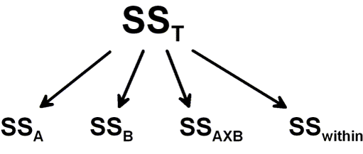
In the first stage of calculations Sum of Squares (SS) Total is calculated and then separated into the two components SS Between Treatments and SS Within Treatments.

In the second stage the SS Between Treatments is separated into the three factors: Factor A, Factor B & Factor A X B (interaction factor)

Source	SS	df	MS	F
Between Treatment (b/t)	SSA + SSB+SSA*B	(kA -1)+ (kB -1)	SSb/t/dfb/t
Factor A	(identify from info. given)	(kA -1)	SSA / dfA	MSA / MSw/i
Factor B	(identify from info. given)	(kB -1)	SSB / dfB	MSB / MSw/i
Interaction	(identify from info. given)	(kA)(kB -1)	SSA*B / dfA*B	MSA*B / MSw/i
Within Treatment (w/i)	SStotal – SSb/t	dftotal – df b/t or N – dfb/t	SSw/i / dfw/i
Total	SSBetween+SSwithin	N – 1

Table 2. ANOVA summary table with calculations

Note: In real life, we would run this through a statistical program with the raw data to calculate the Fs! We are focusing conceptually on calculating the 3 Fs for a two-way factorial ANOVA. Notice that in Table 2, the Sum of Squares Between is adding up the Sum of Squares from each of the factors. You also see that to get to our F-ratios, we need the Mean Squares (just like chapter 14).  We have an F for each: Factor A, Factor B and the Interaction Factor. The calculations for Sum of Square for the factors can be found be knowing the df and MS, or knowing the Sum of Squares Between.

You would also be most likely given the means and standard deviations for the 4 study conditions.  Here is an example from Table 1 (made up data).  You will see the main value as the mean and the standard deviation in parentheses.

Age	Biological sex (male & female)
	Teen Males M = 3.5 (.3)	Teen Females M = 4.5 (.25)
	Older Males           M = 8 (.5)	Older Females M = 12.5 (.8)

Table 2. Means and Standard Deviations example from Table 1 study design.

Possible outcomes for 2-way factorial ANOVA

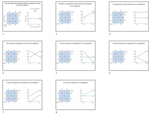
In a 2 X 2 design, there are eight possibilities:

1. A main effect for factor A only
2. A main effect for factor B only
3. Main effects for A and B only
4. A main effect for A, plus an interaction
5. A main effect for B, plus an interaction
6. Main effects for both A and B, plus an interaction
7. An interaction only, no main effects
8. No main effects, no interaction

Figure 1 shows examples of how these findings might look graphing the means of each of the 4 study conditions in a 2×2 design.

Figure 1. Examples of eight outcomes of a 2×2 ANOVA

Make your decision and explain the results (adjusted step 4).

• When making a statistical decision you should begin by looking for patterns in the means from each of the total conditions rather than focusing on the main effects or the interaction. After identifying patterns begin interpreting with the interaction effects first.
• Interaction means that the effect of one factor depends on the level of a second factor – so then there is no consistent main effect. If you get a significant interaction, emphasize that finding over any significant main effects. In other words, if there is an interaction effect, then the main effect cannot be discussed without a qualifier.

Calculate effect size

• Effect size is calculated for each F that is statistically significant.
• Effect size reported is typically eta-square. Remember that from chapter 14, eta-square is the percentage of total variance explained variance by the factor.  Again, just as you have a F for factor A, a F for factor B, and an F for the interaction, you would have eta-squares for each.

Graphing the Results of Factorial Experiments

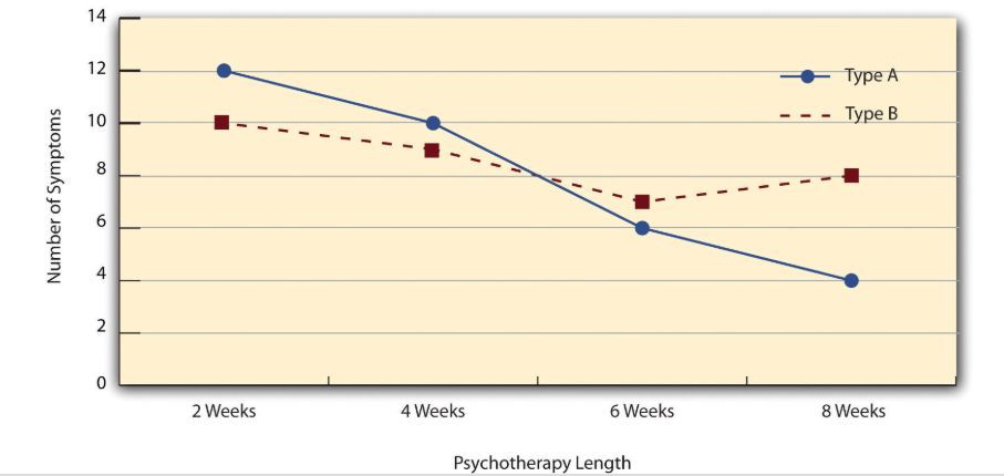
The results of factorial experiments with two independent variables can be graphed by representing one independent variable on the x-axis and representing the other by using different kinds of bars or lines. The y-axis is always reserved for the dependent variable.

Figure 2. A 4 (Psychotherapy Length) x 2 (Type) ANOVA.

The figure above is a line graph that shows results for a hypothetical 4 x 2 factorial experiment Psychotherapy length, is represented along the x-axis and has four levels (e.g., 2 weeks, 4 weeks, 6 weeks and 8 weeks) and the other variable (psychotherapy type) is represented by differently formatted lines.

Advantages & Disadvantages

Considerations

A 2-Factor ANOVA design is relatively easy to carry out and requires fewer subjects than other types of designs. There is no pre-testing necessary because one group could serve as the control. Although identifying sample sizes and study design for power is an important consideration using a factorial ANOVA.

Disadvantages

A 2-Factor ANOVA using a between-subjects design provides little information about the effect of the independent variable. The statistic provides information about whether the two groups differed (on average) and in which direction but it is not sensitive to individual differences.  Other considerations for 2-Factor ANOVAs include using a repeated measures ANOVA.  In this case for a 2-factor ANOVA, each person would be in every condition.  So if you had a 2×2 an individual would be in all 4 study conditions.  Another considerations is having a mixed design.  For a mixed design, one factor would be between-subjects and the other would be within-subjects (repeated measures).  For example, you might wish to conduct a 2×2 study on drug therapy.  You can examine gender differences as one factor and type of drug as the other factor.  Participants are only in 1 gender category but would receive both types of drug.  A mixed design would give you individual differences in how each participant responded to the drug, but also has some of the challenges of using a within-subjects design (see short discussion in chapter 12 on advantages and disadvantages of using a repeated measures design).

Learning Objectives

Having read the chapter, students should be able to:

• Explain the concept of a two-factor research design and recognize a matrix with levels of one factor being rows and levels of the second factor being columns
• Explain main effects and interactions in a two-factor ANOVA including patterns of findings
• Complete a ANOVA table given some information from the study
• Interpret effect size

Exercises – Ch 15

1. True or false. The bigger the differences between the sample means, the more likely it is that at least one of the Fs will be significant.
2. True or false. The advantage of combining two factors into a single research study is that the two factor study provides information about the interaction of the two factors and the main effects of each factor.
3. Complete the ANOVA table given this is a 2×3 ANOVA (two-way ANOVA; factor A = 2 levels with n = 5; factor B = 3 levels with n = 5; N = 30)
   

   Source	SS	df	MS	F
   Between Treatment	60
   Factor A				5
   Factor B
   Interaction	30
   Within Treatment			2
   Total	108

4. What is the df for factor A, B and AxB for the following? What are the corresponding F-critical values?
   1. factor A n=14; factor B n = 18; N = 32

Answers to Exercises – Ch 15

1. true

3.

Source	SS	df	MS	F
Between Treatment	60	5
Factor A	10	1	10	5
Factor B	20	2	10	5
Interaction	30	2	15	7.5
Within Treatment	48	24	2
Total	108	29