Excel Practice 2

Prefer to watch and learn? Check out this video tutorial:

Complete the following Practice Activity and submit your completed project.

For Excel Practice 2, we will use Excel to create an inventory of computer items donated to be refurbished and checked out by students. Key skills in this practice are entering data in a range, using arithmetic operators, quick analysis tool, and absolute and relative cell references,

1. Start Excel. Click Blank Workbook.
2. Select File, Save As, Browse, and then navigate to your Excel folder on your flash drive or other location where you save your files. Name the workbook as Yourlastname_Yourfirstname_Excel_Practice_2.
3. In cell A1, type’ Inventory of Donated Computers and Devices’ and press Enter.
4. Type ‘Items to be Refurbished in cell A2.
5. In cell B3 Type ‘Quantity’ and press Tab. The word Quantity is a label. Labels are used to describe and identify data in a spreadsheet.
6. Type Retail Price and press Tab.
7. Type Additional Cost and press Tab.
8. Type Total Value and press Tab.
9. Type Percent of Total Retail Value and press Enter.
10. In cell A4, type ‘2017 Dell Laptop’ and then press Enter.
11. Apply the autofit to all cells.
12. Select the range A5:A8 and type the following row titles, pressing enter after each one:
    • 2012 Apple iPad
    • 2019 HP Laptop
    • 2020 MacBook Pro
    • Total Value for All Products
13. Notice how when a range is selected, data can be quickly entered by using the enter key.
14. Adjust the width of column A to 420 pixels.
15. Merge and Center the text in the range A1:F1 and then apply the Title style.
16. Merge and Center the text in the range A2:F2 and then apply the Heading 2 style.
17. Check Spelling for the entire worksheet, making necessary corrections. To check the spelling, go to the Review Tab, Proofing group, and choose Spelling. You can also use the shortcut key of F7.
18. Select the range B4:D7.
19. Pressing Enter after each entry with B4 as the active cell, type the following:
    • 10
    • 30
    • 17
    • 7
20. With cell C4 active, continue to type the following values, pressing Enter after each:
    

    Retail Price Additional Cost
    250	82
    200	61
    540	120
    1200	92

21. In cell E4, type =b4*c4 and click Enter. Click in cell E4 and drag the fill handle down to cell E7. Note that the cell reference can be typed in uppercase or lower case when manually typing in a formula. The * is an operator used to multiply two values. In this formula, we are taking the quantity and multiplying it by the retail price to give us the total value.
22. Select the range B4:B7 and apply the comma number style with zero decimals. The comma style is located on the Home Tab, Number Group, Comma. In the same location, click the decrease decimal button twice to remove all decimals.
23. Select the range E4:E7 and notice how at the bottom of your screen, the values for Average, Count, and Sum are displayed. If you right click in this area, you can change the setting to modify what is displayed here.
24. If necessary, select the range E4:E7. Notice in the lower right hand corner of the selected range, the Quick Analysis Tool displays. Using Quick Analysis from the Totals tab, click the first sum button. The sum of the range E4:E7 should display in cell E8.
25. Select the range C4:E8 and cell apply the Accounting number format with zero decimals.
26. In cell E8, apply the Total style.
27. In cell F4, type = click cell E4 type / and then click cell E8. The / is an operator used to divide two values
28. Double-click the formula in cell F4 to display the range finder. This will show you color coded ranges used in the formula. Click Enter.
29. Drag the fill handle on cell F4 down through cell F7.
30. In cell F5, point to the Error Checking button to display the ScreenTip. Notice the divide by zero error. This error means that you are trying to divide by zero, which cannot be done. The denominator is a blank cell with zero content.
31. Double-click the formula in cell F4, and use the F4 key to make the formula absolute so that the new formula is E4/$E$8. Click Enter on the formula bar. Drag the fill handle in cell F4 down to cell F7. If your keyboard does not have the F4 key, you can manually type in the dollar signs. The dollar signs indicate an absolute reference. This means that the denominator will remain at E8, even when the fill handle is used to copy the formula down.
32. Double in cell F5 to show the resulting formula with an absolute reference applied. Notice how the cell E8 has dollar signs.
33. Select the range F4:F7 and format as a percentage with two decimal places.
34. Click cell B5 and type 10, point notice how the other values change.
35. Select the undo button to reverse the last action.
36. Insert a new row above row 3. There are a couple of ways to do this:
    • Click on the 3 row header to select it. Right click and select insert.
    • Click on the 3 row header to select it. On the Home Tab, Cells group, select the arrow next to Insert and select Insert Cells.
37. In cell A3, type As of September 1. Merge and Center the text across the range A3:F3. Apply the Heading 3 Style.
38. Delete column D which contains the additional cost. There are a few ways to do this:
    • Select the D to select the entire column and hit the delete key on your keyboard (you may get a message saying a merged cell cannot be deleted).
    • Select the D to select the entire column, right click and choose Delete.
    • Select the D to select the entire column, on the Home Tab, Cells Group, choose the arrow next to Delete and choose Delete Sheet Columns. Notice how the entire column and the data is deleted and the columns are shifted. The Total Value should be the new column D.
39. Select columns B:F and set the column width to autofit. AutoFit Column Width is found on the Home Tab, Cells Group, and clicking the arrow next to Format.
40. Center the text in the range B5:B8. You may need to change the format to General if the text does not center.
41. Apply Themed Cell Style 20% – Accent 1 to cell A9.
42. On the Page Layout tab, Themes Group, change the theme color to Blue Warm.
43. On the Page Layout tab, Page Setup Group change the orientation to landscape.
44. In Backstage view, show the advanced properties. Add the following:
    • Title: Excel Inventory
    • Subject: BPC110 and Section #
    • Author: Your First and Last Name
    • Keywords: Absolute Reference, Formulas, Excel
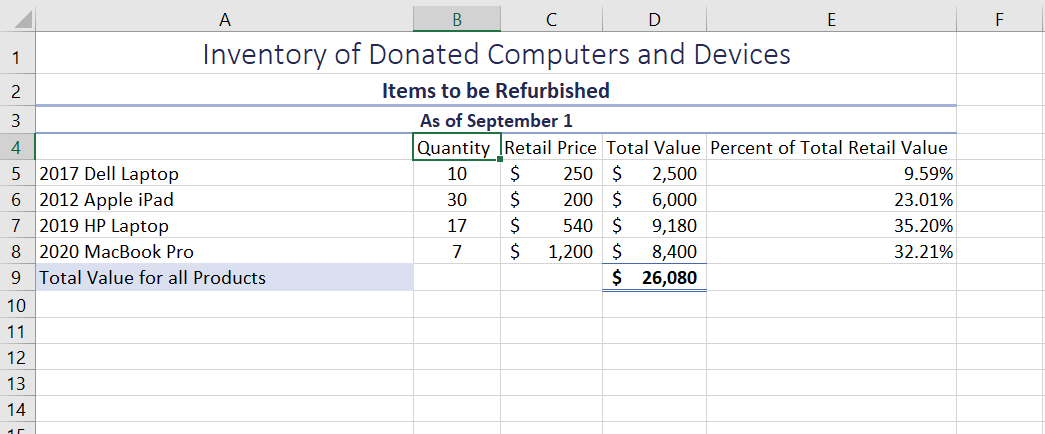
45. Run a spelling and grammar check, compare your file to the image below and make all necessary corrections.
46. Submit as instructed by your instructor