Excel Practice 4

Prefer to watch and learn? Check out this video tutorial:

Complete the following Practice Activity and submit your completed project.

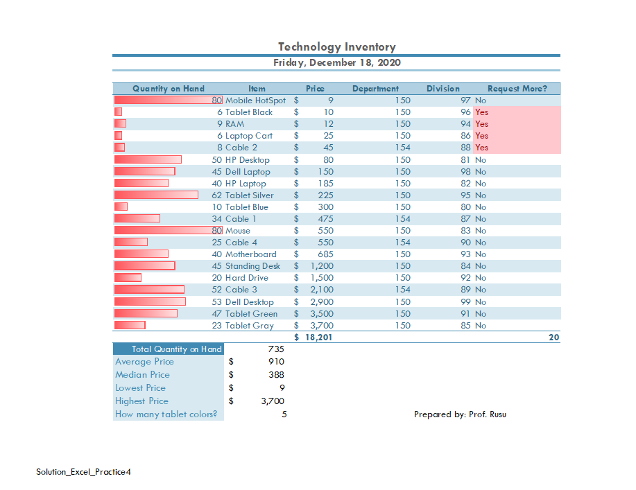
For Excel Practice 4, we will continue to use Excel to manage the technology Inventory at the college. Key skills in this practice are Creating a Summary Sheet, Multiple Worksheets, Headers and Footers.

1. Start Excel. Click Open, then Browse to where your data files are saved. We will continue working on the same spreadsheet as Excel Practice 3.
2. With the Excel Practice 3 open, Select File, Save As, Browse, and then navigate to your Excel folder on your flash drive or other location where you save your files. Name the workbook as Yourlastname_Yourfirstname_Excel_Practice_4.
3. Rename Sheet1 to Inventory. To rename a sheet, right click on Sheet1 and select Rename. Type Inventory and then select Enter.
4. Change the Tab Color to Red, Accent 6. To change the color of the sheet, right click on the sheet name and select Tab Color and then choose Red, Accent 6.
5. Check to see if there is a Sheet2. If not, click the plus button next to the Inventory Sheet. This will add a new blank sheet, called Sheet1. Notice how the sheet names are automatically numbered in sequential order.
6. Rename this sheet to Summary.
7. Change the Tab Color to Aqua, Accent 1.
8. Click the plus button to add another Sheet. Notice how this one is automatically called Sheet2. Right click on Sheet2 and select Delete.
9. On the Inventory tab, in cell A2, change the date format to Long Date. The Data format is on the Home Tab, in the number group. Choose the arrow next to the format window and select Long Date.
10. On the Summary Tab, Type Summary in cell A1 and the press enter. We will use the Summary Tab to create a Summary Sheet.
11. In cell A2, clear the formats. To clear the format, go to the Home Tab, in the Editing Group, choose the arrow next to Clear. Choose Clear All.
12. In cell A2, type Total Quantity and then press Enter.
13. In cell A3, type Average Price and then press Enter.
14. In cell A4 type Highest Price and then press Enter.
15. AutoFit the content of Column A.
16. On the Summary Tab, in Cell B2, type =, then select the Inventory tab and click inside cell B26 and press Enter. This will create a reference from the Summary Sheet to the Inventory Sheet. Verify in cell B2 on the Summary sheet that your formula looks like this: =Inventory!B26. You should see the displayed value of 735 in cell B2 on the Summary Tab.
17. On the Summary Tab, in Cell B3, type =, then select the Inventory tab and click inside cell B27 and press Enter. This will create a reference from the Summary Sheet to the Inventory Sheet. Verify in cell B3 on the Summary sheet that your formula looks like this: =Inventory!B27. You should see the displayed value of 910.05 in cell B3 on the Summary Tab.
18. On the Summary Tab, in Cell B4, type =, then select the Inventory tab and click inside cell B30 and press Enter. This will create a reference from the Summary Sheet to the Inventory Sheet. Verify in cell B4 on the Summary sheet that your formula looks like this: =Inventory!B30. You should see the displayed value of 3700 in cell B4 on the Summary Tab.
19. Select Columns A:B and set the width to 147 pixels.
20. Select the range A1:B1, merge and center the two cells.
21. Select Columns A:F and set the width to 95 pixels.
22. Apply the Heading 1 Cell Style to cell A1.
23. Select the range A2:A4 and apply the Heading 4 style.
24. Select cell B2 and apply the number format with zero decimal places.
25. Select the range B3:B4 and apply the Accounting number format. Ensure there are two decimal places.
26. Click on the Inventory tab, hold the CTRL key, and select the Summary Tab to group the worksheets. Another way to group sheets is to right click on the Inventory tab, and choose Select All Sheets. Notice how the file name across the top of your screen shows [Group].
27. In cell E31, type Prepared by: Your First and Last Name.
28. Double click the Summary Worksheet to ungroup the two sheets. Scroll down to view cell E31 and observe the text in the cell. Display the Inventory Tab, and observe the text in cell E31.
29. Ensure the worksheets are ungrouped by observing the file name. Another way to Ungroup the Worksheets is to right click on one of the tabs and choose Ungroup. It will no longer show [Group].
30. Click in Cell A6 on the Summary Sheet and type HotSpots Available: and press Enter.
31. In cell A7, write a formula that calculates the available HotSpots by taking the Quantity on Hand for Mobile HotSpots from the Inventory worksheet and subtracting 25. The formula in cell A7 should look like this: =Inventory!A5-25
32. Click and hold the summary tab, and drag it to the left of the Inventory tab. The Summary Tab should be first, the Inventory Tab second.
33. With the Summary sheet active, group the worksheets.
34. On the Page Layout Tab, launch the Page Setup dialog box. On the Margins tab, center the worksheets horizontally on the page.
35. IN the Page Setup Dialog box, on the Header/Footer Tab, insert File Name in the left section of the footer. Click OK to close the dialog box.
36. Ungroup the worksheets.
37. In Backstage view, show the advanced properties. Add the following:
    • Title: Excel Technology Inventory 2
    • Subject: BPC110 and Section #
    • Author: Your First and Last Name
    • Keywords: Summary Sheet, Headers and Footers, Grouping Worksheets
    • If necessary, change the Inventory Sheet to Landscape Orientation.
38. Run spelling and grammar check, compare your file to the image below and make all necessary corrections.
39. Submit as instructed by your instructor.