Excel Practice 3

Prefer to watch and learn? Check out this video tutorial:

Complete the following Practice Activity and submit your completed project.

For Excel Practice 3, we will use Excel to manage the technology Inventory at the college., where you work as a Data Analyst. Key skills in this practice are Flash Fill, Advanced Functions, and Conditional Formatting.

1. Start Excel. Click Open, then Browse to where your starter files are located. Open the starter file Starter_Excel_Practice3.
2. With the file open, Select File, Save As, Browse, and then navigate to your Excel folder on your flash drive or other location where you save your files. Name the workbook as Yourlastname_Yourfirstname_Excel_Practice_3.
3. We will use Flash Fill to separate the date in column D. In cell E4, type Department and then press Tab. In cell F4 type Division and then press enter. These are our column labels for the flash fill.
4. In cell E5 type 150 and press enter. With cell E6 as the active cell, go to the Home Tab, Editing Group, Choose the arrow next to Fill and Choose Flash Fill. Notice how the contents from column D are automatically filled to column E, and only the Department was filled.
5. With cell F5 as the active cell, type 80 and press enter. With cell F6 selected, press the shortcut key for Flash Fill – Ctrl + E. Notice how the two-digit division code was filled for column F.
6. Delete column D.
7. AutoFit columns B through E. If necessary deselect wrap text before auto fitting.
8. Merge and Center cell A1 across the range A1:F1. Then apply the Heading 1 cell style.
9. Merge and Center cell A2 across the range A2:F2. Then apply the Heading 2 Style.
10. Select cell B26. On the Formulas Tab, in the function library group, choose Insert Function and search for the SUM function, select Go and then select OK. Apply the SUM function to the range A5:A24. Before searching for the SUM function in the Search Box, you may need to clear out any existing text.
11. Click cell B27, and using the same method as above apply the AVERAGE function to the range C5:C24.
12. Click in cell B28, and using the same method, apply the MEDIAN function to the range C5:C24.
13. Click cell B29, and using the same method apply the MIN function to the range C5:C24.
14. Click cell B30, and using the same method apply the MAX function to the range C5:C24.
15. Select the range B27:B30 and apply the Accounting Number Format with no decimal places.
16. Select column C and set the width to 50 pixels.
17. ## symbols should display in some of the cells in column C. This means that the column is not wide enough to display the underlying value. Select columns B:C and AutoFit the columns. Notice how the ## go away and the underlying value displays.
18. Select the range A4:F4 and apply the 40% – Accent 1 Themed cell style and center the text.
19. Select cell A26, change the font size to 14, apply Bold and Italic, and select the Accent 1 Cell Style under Themed Cell Styles. Align-right the text.
20. Select the range A27:A30 and on the Home Tab, Cells Group, choose the arrow next to Format and launch the Format Cells dialog box at the bottom of the list. On the Font Tab, choose 12 for the Size, and Blue Accent 1 for the Color:

• • On the Fill tab choose the second light blue color (any light blue color will work)
  • Select OK to exit out of the dialog box

21. In cell A31 type “How many tablet colors?”.
22. In Cell B31, we will write a formula to count the Item Names if it contains the work Tablet. This will tell us how many different tablet colors we have. We will use the COUNTIF function to do this:

• • With cell B31 active, go to the Formulas Tab, in the Function Library choose Insert Function.
  • Search for COUNTIF, select it, and then select Go.
  • In the Function Arguments dialog box, in the Range box, select the range B5:B24. This range represents the Item Names. You can type in the range, or move the dialog box to the side and select it.
  • In the Criteria box, type the word ‘Tablet*” and click OK. It is important to include the asterisk after the word Tablet. The asterisk represents a wildcard.

23. In cell F4, type Request More?, and autofit the cell width.
24. In cell F5, we will write an IF statement to determine if we need to request additional items because the stock is running low. If there are less than 10 items on hand, we need to request more.

• • With cell F5 active, go to the Formulas tab, in the Function Library choose Insert Function.
  • Search for “IF”, select it, and then choose Go.
  • In the Function Arguments dialog box, next to Logical_test, enter A5<10
  • Next to Value_if_true, enter Yes.
  • Next to value_if_false enter No.
  • Select Ok to exit out of the dialog Box.
  • In cell F5, you should see the word No display. This is because there are 10 Blue Tablets on hand so we do not need to request more.
  • With cell F5 still active, use the fill handle to copy the IF statement to cell F24.

25. Select the range F5:F24. On the Home Tab, in the Styles Group, choose the arrow next to Conditional Formatting, and apply the Highlight Cell Rules using Text that Contains the word Yes. Choose the default formatting with Light Red Fill with Dark Red Text.
26. Select the range A5:A24. On the Home Tab, in the Styles Group, choose the arrow next to Conditional Formatting and apply Data Bars using a Red Gradient Fill Data Bar.
27. Make cell A2 the active cell by typing A2 in the Name box.
28. On the Home Tab, in the Editing Group, choose the arrow next to Clear and choose clear contents. This will clear any data in the cell, but keep the format.
29. In cell A2 Insert the NOW function. There are several ways to do this:

• • In the formula bar, type =NOW()
  • On the Formulas tab, in the Function Library group, choose the arrow next to Data & Time. Choose NOW and then Enter.
  • On the Formulas tab, in the Function Library group, choose Insert Function. Search for the NOW function and choose Go. Select NOW and then OK, and OK again.

30. Select the range A4:F24.
31. On the Insert tab, tables group, choose Table. Check the box that says My Table has Headers and then click OK.
32. On the Table Tools, Design Tab, choose Quick Styles. Select the third quick style in the first row, Table Style Light 2.
33. Sort the Retail Price from Smallest to Largest. Click the arrow next to Price in cell C4, and choose sort smallest to largest.
34. Select the range C5:C24, format as currency with zero decimal places and autofit the cell contents.
35. Choose the arrow next to Department, and Filter the Department so only 150 shows.
36. Add a Total Row to the table. On the Table Tools Design tab, choose the check box next to Total. Notice that since the Department field is still filtered, there are 16 records with a department of 150.
37. Remove the filter on department by clicking the arrow next to the word department, and choosing select all. Notice how the total now shows 20.
38. Click cell C25, click the arrow that displays to the right, and select Sum. Notice how this adds together the Price column to display a grand total.
39. On the Page layout tab, in the Themes group, select the arrow net to Themes and apply the Integral Theme. Change the colors to Marquee.
40. On the Page Layout tab, in the page setup group, change the orientation to landscape and center on the page horizontally.
41. Select the range A25:F25, apply the Heading 4 style and apply Center alignment.
42. Press Ctrl + F2 to display Print Preview.
43. In Backstage view, show the advanced properties. Add the following:
    • Title: Excel Technology Inventory
    • Subject: BPC110 and Section #
    • Author: Your First and Last Name
    • Keywords: Functions, Conditional Formatting, Tables

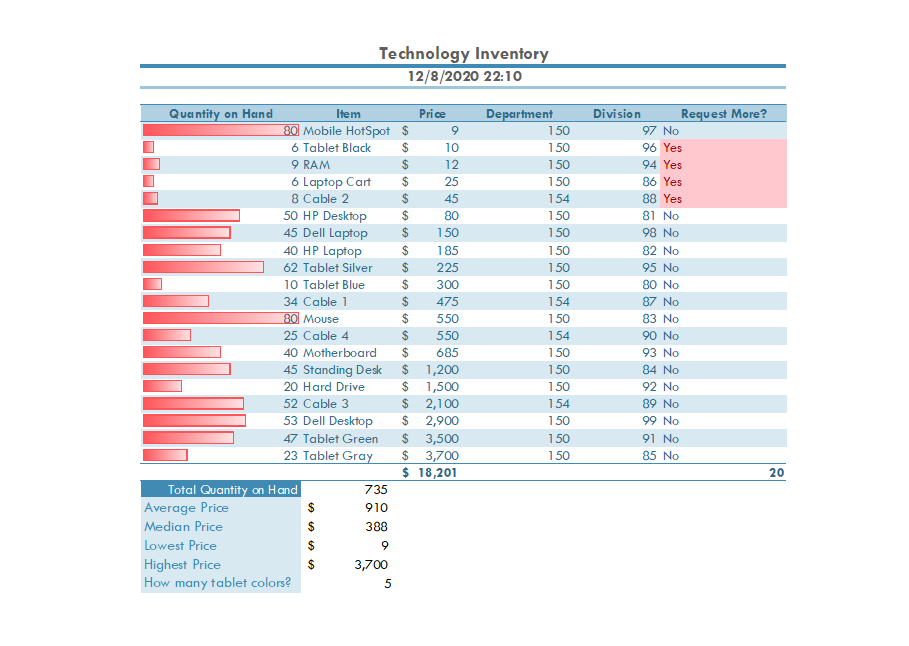
44. Run spelling and grammar check, compare your file to the image below and make all necessary corrections.
45. Submit as instructed by your instructor.