Creative Commons Attribution for Text

​(1) An Introduction to Geology by Chris Johnson, Matthew D. Affolter, Paul Inkenbrandt, Cam Mosher is licensed under CC BY-NC-SA 4.0

(2) Geology by Lumen Learning is licensed under CC BY-NC-SA 4.0

(3) Earth Science by Lumen Learning is licensed under CC BY-NC-SA 4.0

(4) Natural Disasters and Human Impacts by R. Adam Dastrup, MA, GISP is licensed under CC BY-NC-SA 4.0

(5) Physical Geology – 2nd Edition by Steven Earle is licensed under CC BY 4.0.

(6) United States Geological Survey (USGS) is licensed under Public Domain.

Media Assets

5.0

Video 5.1.  Arizona Geological Survey (2011) Time lapse: Historic earthquake epicenters of Arizona.  [Online video]. Retrieved April 19, 2021 from https://youtu.be/TjgLe0hCWXw

• Time lapse video of historical earthquakes that have occurred in Arizona 1852-2011

5.1

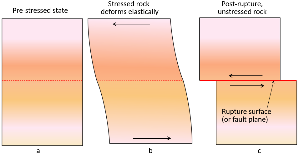
Fig. 5.1.1.  Earle, S. (n.d.) Physical Geology – 2nd Edition.  Depiction of elastic deformation and rupture.  Retrieved April 19, 2021 from https://opentextbc.ca/physicalgeology2ed/wp-content/uploads/sites/298/2019/06/elastic-deformation.png

• Depiction of the concept of elastic deformation and rupture.

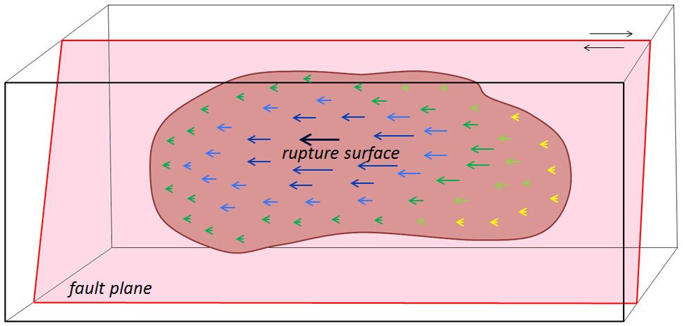
Fig. 5.1.2.  Earle, S. (n.d.) Physical Geology – 2nd Edition.  Propagation of failure on rupture surface.  Retrieved April 19, 2021 from https://opentextbc.ca/physicalgeology2ed/wp-content/uploads/sites/298/2019/08/Propagation-of-failure.png

• Image showing the direction and magnitude of ruptures along the rupture surface during an earthquake

Video 5.1.3.  United States Geological Survey, (n.d.) Foreshocks, Mainshocks, & Aftershocks.  https://prd-wret.s3.us-west-2.amazonaws.com/assets/palladium/production/s3fs-public/atoms/video/aftershocks.mp4.  Public Domain

• Video showing foreshocks, mainshocks, and aftershocks locations along the rupture surface.

Fig. 5.1.4. Wikimedia Commons (March, 2011)).  Map of Sendai Earthquake.  Retrieved April 19, 2021 from https://en.wikipedia.org/wiki/2011_T%C5%8Dhoku_earthquake_and_tsunami#/media/File:Map_of_Sendai_Earthquake_2011.jpg

• Map of main earthquake event and subsequent aftershocks in the following 3 days.

Fig. 5.1.5. NASA (n.d.) Lunar Fault Scarp.  Retrieved April 19, 2021 from https://www.nasa.gov/sites/default/files/styles/full_width/public/thumbnails/image/press_image_1_v2.jpg?itok=tvHkaaC0

• Image of a fault scarp in the moon.

5.2

Fig. 5.2.1.  Christiansen, L (n.d.) A global map of seismic activity.  Retrieved April 19, 2021 from https://www.nsf.gov/news/mmg/media/images/global_seismicity_h.jpg

• An image showing the pattern and depth of global earthquake activity.

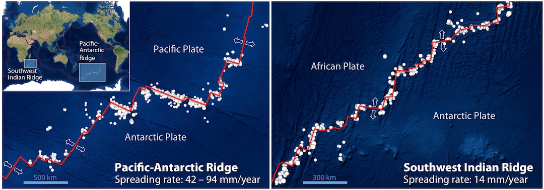
Fig. 5.2.2. Panchuk, K. (2017)  Locations of earthquakes of magnitude 4 and greater from 1990 to 2010 along two mid-oceanic ridges. Retrieved April 19, 2021 from https://openpress.usask.ca/app/uploads/sites/29/2017/11/Div_Trans_Eq.png

• Image showing the relationships of earthquakes along divergent and transform boundaries. Arrows show the direction of plate movement.

Fig. 5.2.3. USGS (n.d) San Andreas Fault.  Retrieved April 19, 2021 from https://upload.wikimedia.org/wikipedia/commons/7/76/Sanandreas.jpg

• Map of the San Andreas fault showing plate motions.

Fig. 5.2.4. Earle, S (n.d.) Physical Geology – 2nd Edition. Retrieved April 19, 2021 from https://opentextbc.ca/physicalgeology2ed/wp-content/uploads/sites/298/2019/08/subduction-quakes.png

• Distribution of earthquakes of M4 and greater in the Central America region from 1990 to 1996

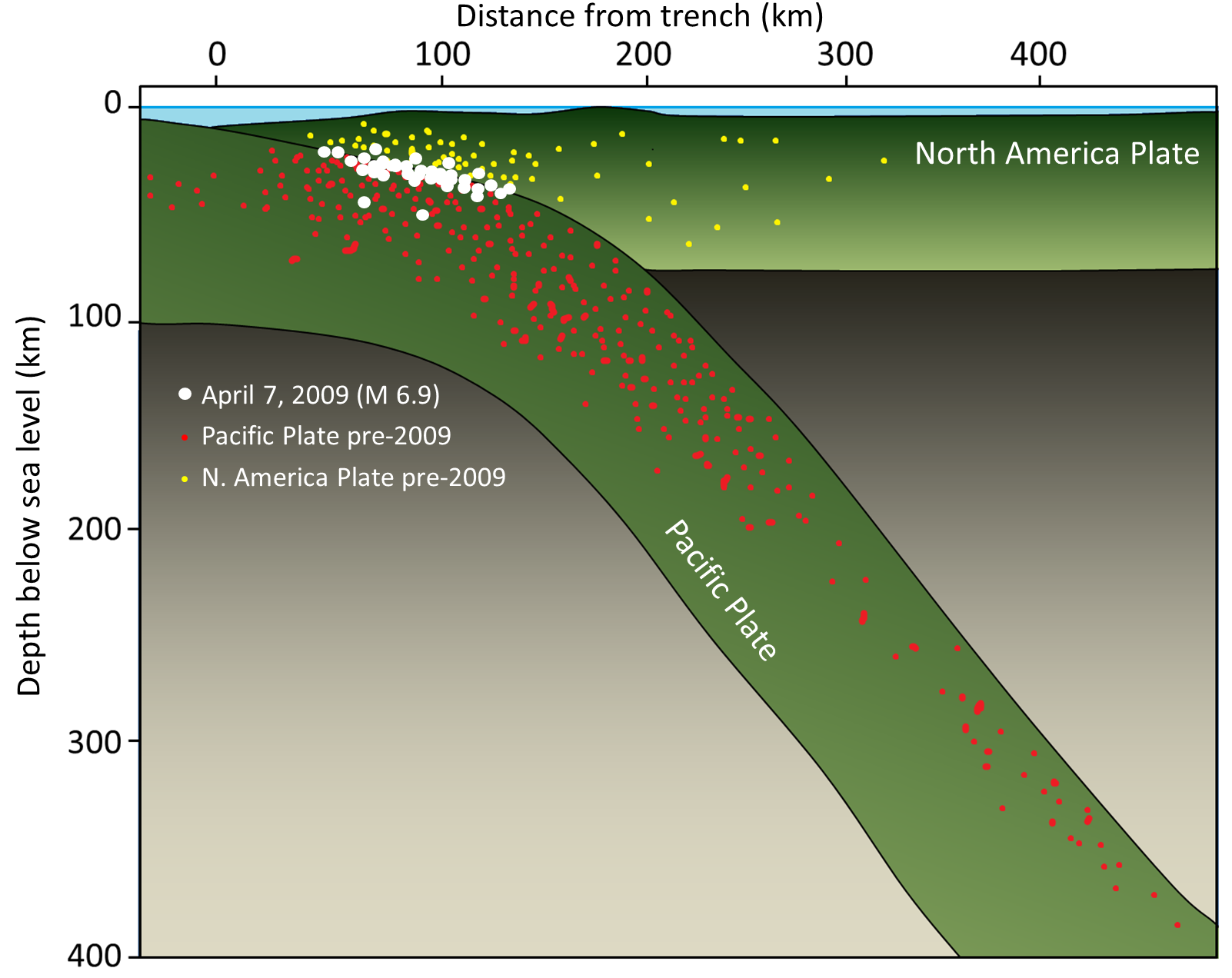
Fig. 5.2.5. Earle, S (n.d) Physical Geology – 2nd Edition.  Retrieved April 19, 2021 from https://opentextbc.ca/physicalgeology2ed/wp-content/uploads/sites/298/2019/08/Kuril-Islands.png

• Graphic of cross-sectional view of distribution of earthquakes of M4 and greater in the Central America region from 1990 to 1996.

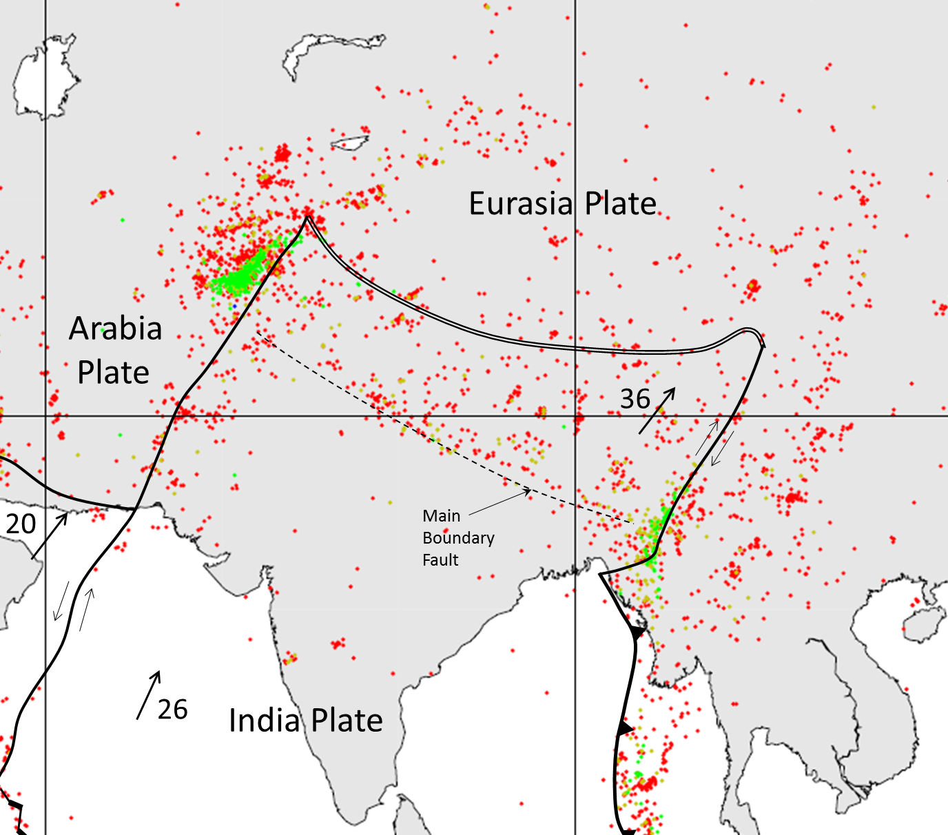
Fig. 5.2.6. Earle, S (n.d) Physical Geology – 2nd Edition.  Retrieved April 19, 2021 from https://opentextbc.ca/physicalgeology2ed/wp-content/uploads/sites/298/2019/08/India-Plate.png

• Figure showing distribution of earthquakes in the area where the India Plate is converging with the Asia Plate.

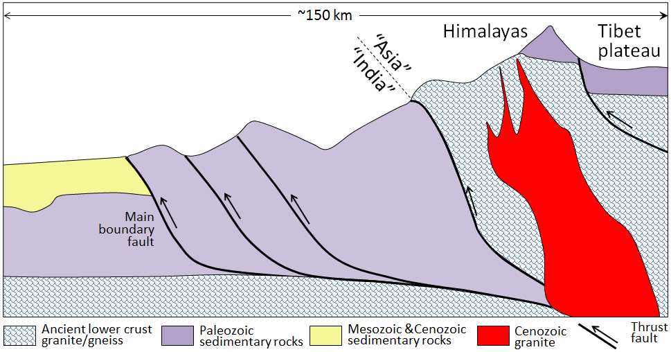
Fig. 5.2.7. Earle, S (n.d) Physical Geology – 2nd Edition.  Retrieved April 19, 2021 from https://opentextbc.ca/physicalgeology2ed/wp-content/uploads/sites/298/2019/08/India-Asia-convergent-boundary.png

• Schematic diagram of the India-Asia convergent boundary, showing examples of the types of faults along which earthquakes are focused. The devastating Nepal earthquake of May 2015 took place along one of these faults.

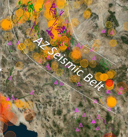
Fig. 5.2.8. Arizona Geological Survey (n.d.) AZ Seismic Belt.  Retrieved April 19, 2021 from https://azgs.arizona.edu/sites/default/files/styles/azgs_optimized_large/public/NAZ%20seismic%20zone%20labeled.jpg?itok=BYD6Rifv

• Map showing the distribution of major earthquakes across Arizona.

5.3

Fig. 5.3.1. Utah Geologic Survey (n.d.) Focus and Epicenter.  Retrieved April 19, 2021 from https://geology.utah.gov/wp-content/uploads/svnt47-3_eq_early_warning_sys.gif

• Schematic showing the relationship between the focus, earthquake, and fault scarp.

Fig. 5.3.2. Panchuck, K (2018).  Retrieved April 19, 2021 from https://openpress.usask.ca/app/uploads/sites/29/2018/01/body_waves.png

• Image showing seismic waves simulated using a spring and rope attached to a fixed surface. Top: P-waves travel as pulses of compression. Bottom: S-waves move particles at right angles to the direction of motion

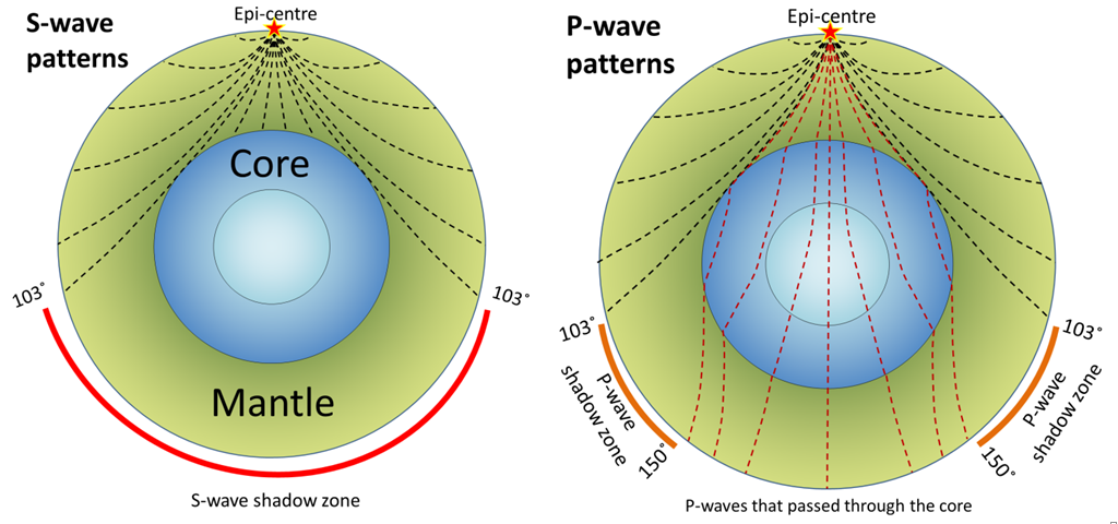
Fig. 5.3.3. Earle, S (2016) Retrieved April 19, 2021 from https://openpress.usask.ca/app/uploads/sites/29/2018/03/shadow-2-SE.png

• Image showing patterns of seismic wave propagation through Earth’s mantle and core. S-waves do not travel through the liquid outer core, so they leave a shadow on Earth’s far side. P-waves do travel through the core, but because the waves that enter the core are refracted, there are also P-wave shadow zones.

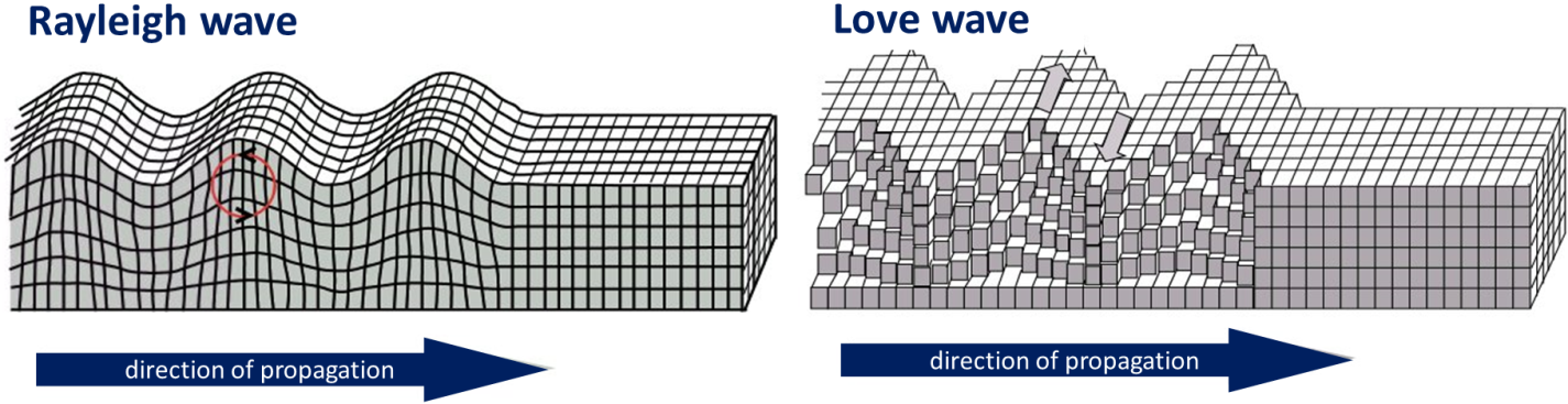
Fig. 5.3.4. Earle, S (2015).  Retrieved April 19, 2021 from https://openpress.usask.ca/app/uploads/sites/29/2017/05/seismic-surface.png

• Image showing surface waves, which travel along Earth’s surface and have a diminished impact with depth. Rayleigh waves (left) cause a rolling motion, and Love waves (right) cause the ground to shift from side to side.

Fig. 5.3.5. Wikimedia Commons (November, 2018)  Seismograph Recording.  Retrieved April 19, 2021 from https://commons.wikimedia.org/wiki/File:Seismograph_recording.jpg

• Image of Seismograph showing seismogram

Fig. 5.3.6. Wikimedia Commons (2011). Retrieved April 19, 2021 from https://live.staticflickr.com/5299/5520554611_1f2b88c5ef_b.jpg

• Image showing multiple seismographs combined to show the dramatic movements from the magnitude 9.0 earthquake, Japan, 2011.

Fig. 5.3.7. USGS (n.d.) Retrieved April 19, 2021 from https://prd-wret.s3.us-west-2.amazonaws.com/assets/palladium/production/s3fs-public/styles/full_width/public/thumbnails/image/eq-ed-triangulation.gif

• Image showing how Triangulation can be used to locate an earthquake.

Video 5.3.1. Geoscience Australia (May 18, 2020) Earthquake monitoring. Retrieved April 19, 2021 from https://youtu.be/GcNVpMZlIDo

• Video showing how earthquakes are monitored and how seismic waves are measured.

Fig. 5.3.8.  USGS (n.d.) Modified Mercali Intensity Scale.  Retrieved April 19, 2021 from https://www.usgs.gov/media/images/modified-mercalli-intensity-scale

• Image showing the Modified Mercalli Intensity Scale.

Fig. 5.3.9  Wikimedia Commons (2007) Earthquake severity.  Retrieved April 19, 2021 from https://commons.wikimedia.org/wiki/File:Earthquake_severity.jpg

• Image showing the relative size of the earthquake and severity.

Video 5.3.2. Incorporated Research Institutions for Seismology (n.d.) Retrieved April 19, 2021 from https://www.iris.edu/hq/inclass/uploads/videos/A_004A_momentmagnitude.mp4?_=1

• Video showing the difference between the Richter Scale and Moment Magnitude

Fig. 5.3.10  Arizona State Geological Survey (n.d.) Retrieved April 19, 2021 from https://azgs.arizona.edu/sites/default/files/styles/azgs_optimized_large/public/azgs-photo-gallery/IMG_0004.JPG?itok=PGJux2hU

• Image showing a research geologist uncovering a seismic station in Southern Arizona.

5.4

Fig. 5.4.1 USGS (n.d.) Retrieved April 19, 2021 from https://earthquake.usgs.gov/learn/glossary/images/amplification.jpg

• Map of amplification potential in Los Angeles

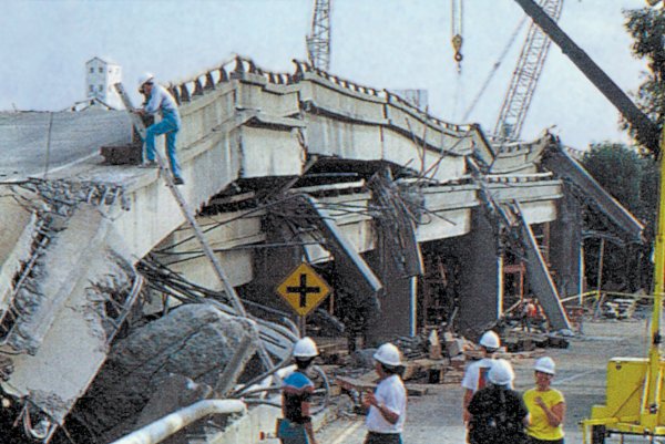
Fig. 5.4.2 USGS (n.d) Retrieved April 19, 2021 from https://upload.wikimedia.org/wikipedia/commons/9/91/Cypress_collapsed.jpg

• Image of the Cypress Structure, the freeway approach to the Bay Bridge, which collapsed during the Loma Prieta earthquake, killing 42 people.

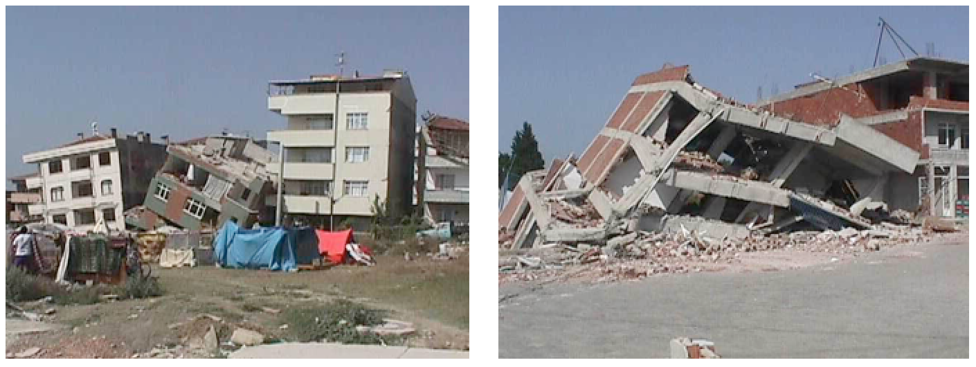
Fig. 5.4.3 USGS (n.d.) Retrieved April 19, 2021 from https://opentextbc.ca/physicalgeology2ed/wp-content/uploads/sites/298/2019/08/earthquake-in-the-Izmit.png

• Images of Buildings Damaged by the 1999 Earthquake, Izmit, Turkey.

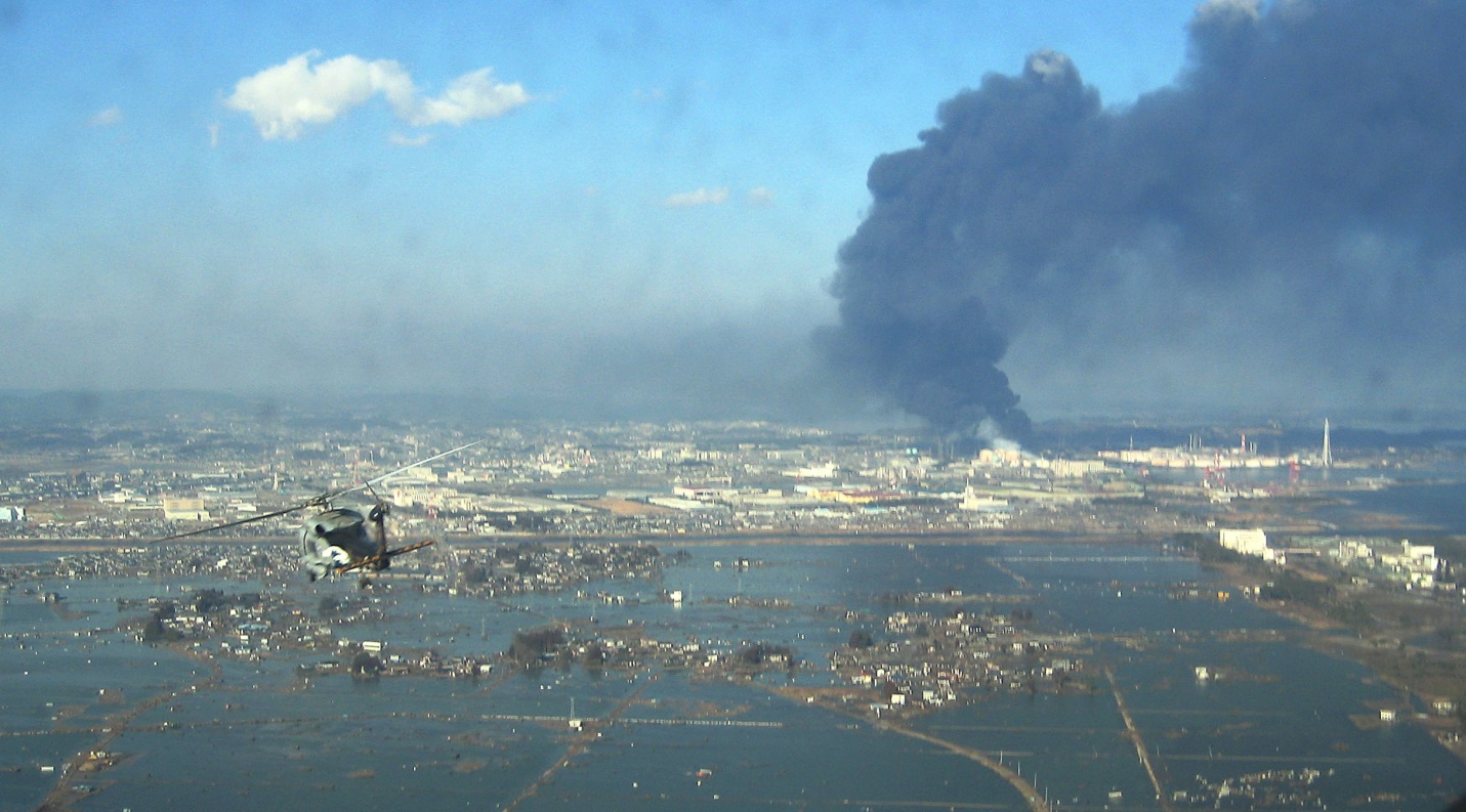
Fig. 5.4.4  United States Navy (n.d.) Retrieved April 19, 2021 from https://opentextbc.ca/physicalgeology2ed/wp-content/uploads/sites/298/2019/08/Tohoku-earthquake.jpg

• Photograph of effects of the 2011 Tohoku earthquake in the Sendai area of Japan.

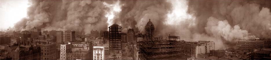
Fig. 5.4.5  Library of Congress (n.d.) San Francisco Fire.  Retrieved April 19, 2021 from https://opentextbc.ca/physicalgeology2ed/wp-content/uploads/sites/298/2019/08/Fires-in-San-Francisco.jpg

• Photograph of San Francisco Fire, 1906

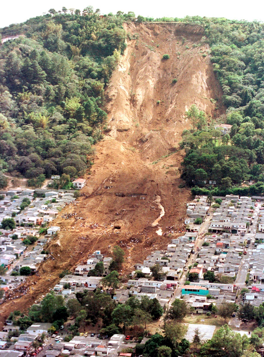
Fig. 5.4.6 USGS (n.d.) Retrieved April 19, 2021 from https://opentextbc.ca/physicalgeology2ed/wp-content/uploads/sites/298/2019/08/The-Las-Colinas-debris.jpg

• The Las Colinas debris flow at Santa Tecla (a suburb of the capital San Salvador) triggered by the January 2001 El Salvador earthquake.

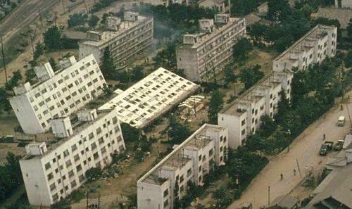
Fig. 5.4.7 Wikimedia Commons (n.d.) Retrieved April 19, 2021 from https://opentextbc.ca/physicalgeology2ed/wp-content/uploads/sites/298/2019/08/Niigata.jpg

• Aerial photograph of damage due to liquefaction from earthquake in Japan, 1964

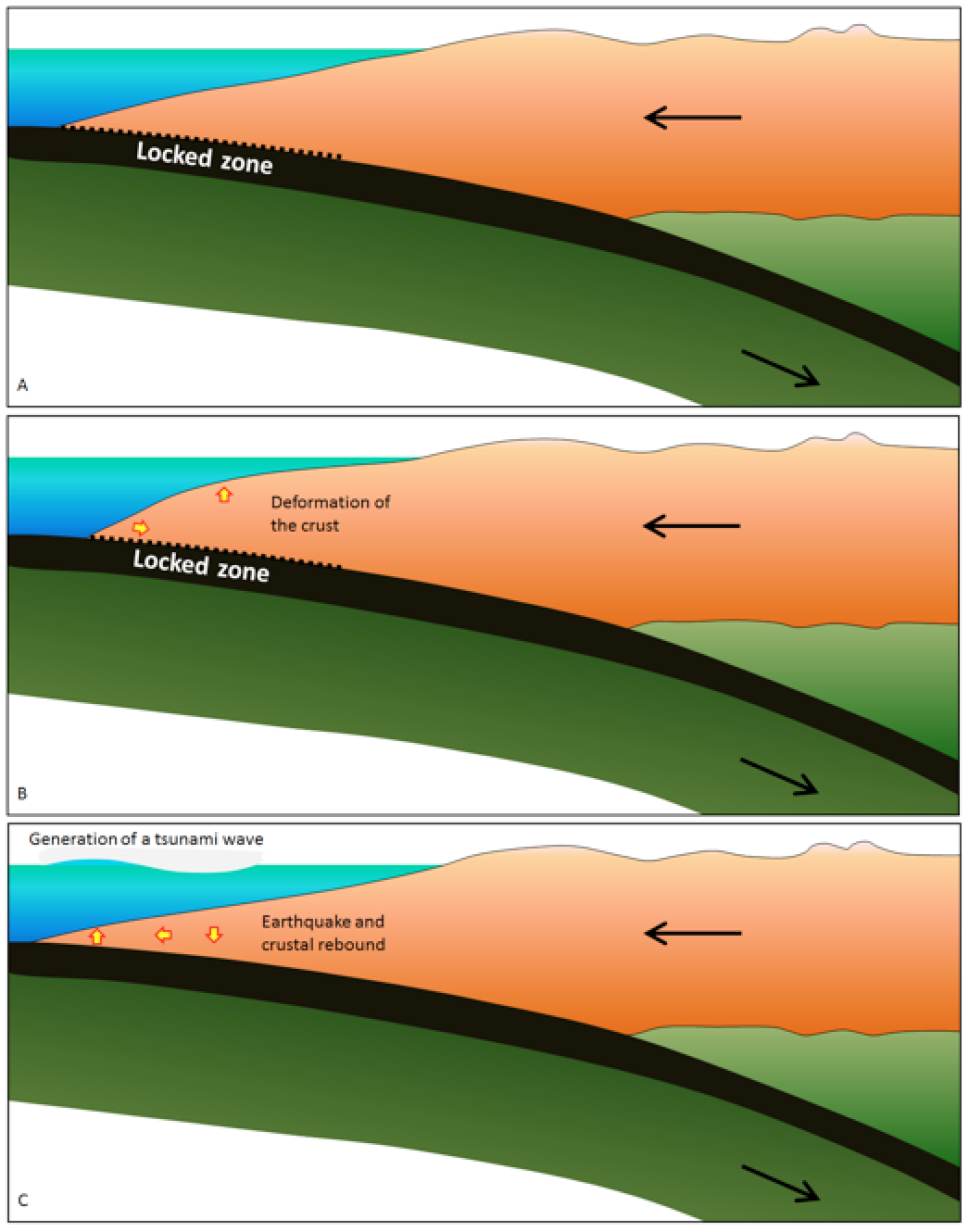
Fig. 5.4.8 Earle, S.  (n.d.) Retrieved April 19, 2021 from https://opentextbc.ca/physicalgeology2ed/wp-content/uploads/sites/298/2019/08/Elastic-deformation.png

• Figure of elastic deformation and rebound of overriding plate at a subduction setting

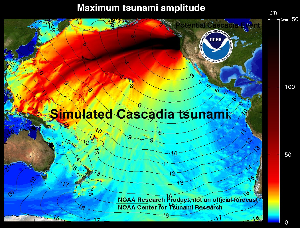
Fig. 5.4.9  NOAA (n.d.) Retrieved April 19, 2021 from https://opentextbc.ca/physicalgeology2ed/wp-content/uploads/sites/298/2019/08/tsunami.png

• Image of Maximum Tsunami Amplitude. A model of the tsunami wave heights (colors) and travel time contours from the 1700 Cascadia earthquake (M9).

5.5

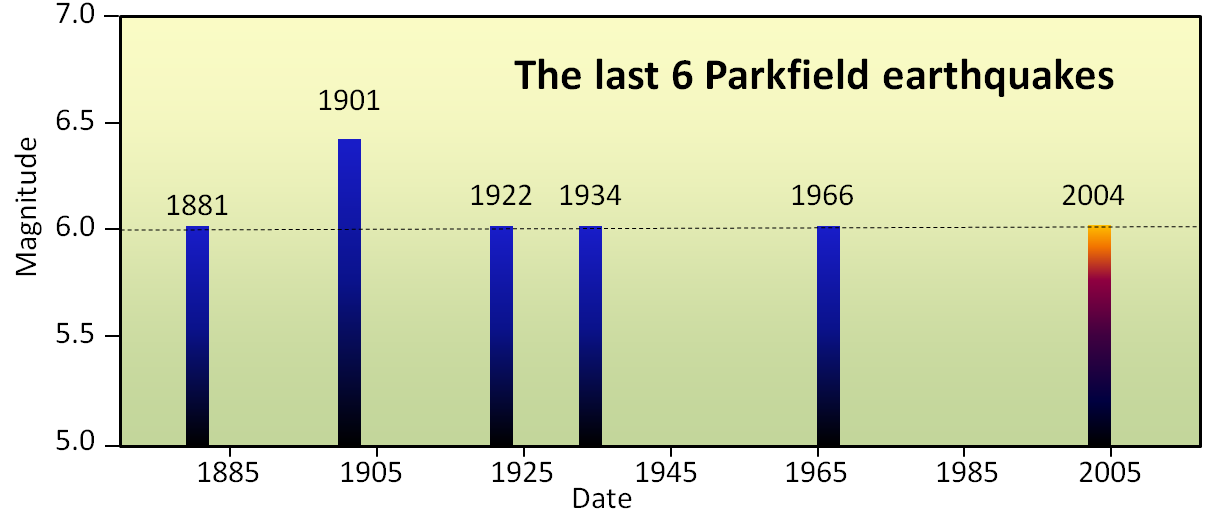
Fig. 5.5.1 Earle, S (n.d.) Retrieved April 19, 2021 from https://opentextbc.ca/physicalgeology2ed/wp-content/uploads/sites/298/2019/06/Parkfield-segment.png

• Graph showing relative numbers of earthquakes on the Parkfield segment of the San Andreas.

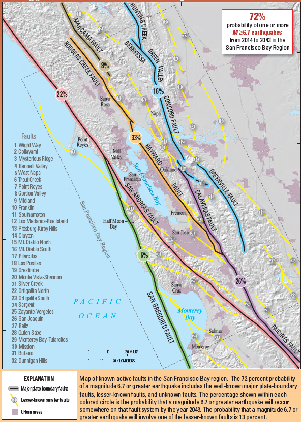
Fig. 5.5.2 USGS (n.d.) Retrieved April 19, 2021 from https://opentextbc.ca/physicalgeology2ed/wp-content/uploads/sites/298/2019/08/bay-area-prob.png

• Map showing probabilities of a M6.7 or larger earthquake over a period of 2014-2043 on various faults in the San Francisco Bay region of California.

Video  5.5.1. Arizona State Geological Survey (2013) Lake Mary Fault, Arizona.  Retrieved April 19, 2021 from https://youtu.be/vi3TVP8l7rc

• Video showing the development of the Lake Mary Fault system, Arizona.

Instructor Resources

DP22_Ch05_Earthquakes Text only